Concentration and the Central Limit Theorem Explained: How Many Samples Your Number Needs
The error bar for practitioners: why an average of independent, identically distributed draws has a Gaussian error of size sigma over root n and how fast that becomes true, why a mean of rare events needs a hundred times more data than a symmetric one, what Chebyshev, Hoeffding and the exact binomial each know, how many test examples resolve a one-point gap (about 12,000 unpaired, a few hundred disagreements paired), why picking the best of a hundred checkpoints adds three points you did not earn, why random vectors in 4,096 dimensions are nearly orthogonal and attention divides by root d, and why 10,000 correlated samples can be worth 50 independent ones — with the batch-means fix.
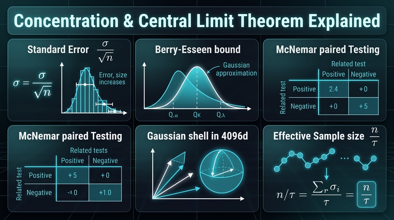
Prerequisites: random variables, expectation, variance and independence at the level of this week's other explainer, Probability Theory Explained, in particular its §5 on the two limit theorems. Everything here is a consumer of those.
Reading path. On a first pass the core is §1 (the three questions), §2 (the central limit theorem and its speed), §4 (the eval-set error bar, with the table) and §6 (correlated samples). §3 (the inequalities, and what each one knows) and §5 (high dimensions) are the parts that explain why the numbers in §4 and §6 are what they are, and §7 collects the traps. If you came here for one number, it is in §4.2: about test examples per model for an observed one-point accuracy difference between two models to be two-sigma unpaired at accuracy (about to plan a test that detects one with power), or a few hundred disagreements paired.
Companion Notebook
This article pairs with 01_concentration_and_chains.ipynb — pure NumPy and Matplotlib, CPU-only, every figure inline — which ships with this piece and carries the same material in runnable form: the dice sums converging to a bell, the characteristic function doing the proof's work, the Berry–Esseen gap measured against its bound, the heavy-tailed block means that never become Gaussian, the three inequalities against the exact binomial, interval coverage measured as a frequency, the eval-set and pairing tables, the selection-bias curve, the geometry of random vectors in , and an AR(1) chain and a Metropolis sampler with their effective sample sizes. Every table and printed block quoted below is copied line-for-line from the output of worked_numbers_companions.py (sections §B1–§B21), the script the notebook is built from — Python 3.14.5, NumPy 2.5.3, float64, seed 20261029 fixed at the top — so a re-execution reproduces every one of them; a few sections are quoted in part, but no quoted line is edited, and values derived from those outputs in the prose are marked where they appear.
1. Three questions with one answer
Three things happen in a working week that look unrelated.
A colleague reports that the new checkpoint scores on the benchmark against the old one's , on examples, and asks whether to ship it. A retrieval system over a million embeddings in dimensions returns the right document with a dot product of and the wrong ones near zero, and someone asks why that works when a million vectors "should" crowd each other. And a sampler — an MCMC chain, a long reinforcement-learning rollout, a sequence of per-token losses — produces numbers whose average someone wants to quote with a standard error of .
All three are questions about how a sum of random quantities behaves, and all three have the same answer in two parts. The first part is the central limit theorem: a sum of many independent, identically distributed terms with finite variance is close to Gaussian, with spread for the sum and for the mean. The second part is concentration: how close, at finite , with a bound you can write down — and what changes when the terms are rare events, when there are many sums to pick from, when the "sum" is a dot product in a high-dimensional space, or when the terms are not independent. The benchmark gap is a difference of two sample means. The retrieval scores are dot products, which are sums of terms. The chain average is a sum of correlated terms. §2 to §6 take them in that order.
2. The central limit theorem, and how fast it arrives
2.1 The statement, and what it looks like
Take independent, identically distributed draws with mean and variance . The central limit theorem says that the standardised sum
converges in distribution to a standard Gaussian: for every . Equivalently, the sample mean is approximately . Nothing is assumed about the shape of the beyond the hypotheses just stated — independent, identically distributed, with a finite and positive variance; a die, a coin, a per-example loss and a reward all qualify. Here is a die, flat on six values and nothing like a bell:
§B1 n =  1: sup |F_n - Phi| = 0.1434 (Kolmogorov distance);  continuity-corrected gap at k + 1/2 = 0.0542;  P(mean within ±0.5 of 3.5) = 0.3333
    n =  2: sup |F_n - Phi| = 0.0833 (Kolmogorov distance);  continuity-corrected gap at k + 1/2 = 0.0164;  P(mean within ±0.5 of 3.5) = 0.4444
    n =  5: sup |F_n - Phi| = 0.0525 (Kolmogorov distance);  continuity-corrected gap at k + 1/2 = 0.0054;  P(mean within ±0.5 of 3.5) = 0.5571
    n = 30: sup |F_n - Phi| = 0.0214 (Kolmogorov distance);  continuity-corrected gap at k + 1/2 = 0.0009;  P(mean within ±0.5 of 3.5) = 0.9025
The first column is the Kolmogorov distance — the largest gap anywhere between the true distribution function of the standardised dice mean and the Gaussian's, computed exactly from the convolution of six-point distributions and checked on both sides of every jump, since a lattice distribution function jumps at the integers and the Gaussian's does not; the sup sits at a jump, so an evaluation at the atoms alone would miss it. It is for one die and still at thirty — the quantity Berry–Esseen (§2.3) bounds, and it shrinks like , not faster. The second column is what a careful practitioner's half-step continuity correction buys (evaluate at rather than at ): a grid discrepancy at the atoms, not a sup over all , and it is an order of magnitude smaller — by five dice the corrected Gaussian is within half a percent at every atom, by thirty within a tenth of a percent. Read the two columns together: the Gaussian approximation to a lattice sum is good only with the continuity correction, and the uncorrected distance is what a theorem about sees. The third column is the law of large numbers made visible — the mean of thirty dice is within half a pip of ninety percent of the time.
Three statements about the same average, in three different modes, license three different things. The modes are ordered — almost sure implies in probability implies in distribution — and the CLT's is the weakest of the three; but the statements are not ordered, because the CLT is about a finer object, the rescaled error rather than the mean itself, which is exactly why it is the one that yields an error bar:
| Statement | Mode | What it licenses | What it does not |
|---|---|---|---|
| with probability one (strong law) | almost surely | your running mean settles at | any rate, or any error bar |
| (weak law) | in probability | the chance of a large error at step vanishes | that your particular run's error vanishes |
| (CLT) | in distribution | the error bar and its Gaussian shape, as a frequency over repetitions | anything about one path, or about how good the approximation is at a given — that needs a rate (§2.3) |
2.2 Why it is true, in one paragraph
The proof is short enough to state and it explains the theorem rather than merely establishing it. The characteristic function of a random variable is — the Fourier transform of its distribution. Independence turns the sum's characteristic function into a product of the terms' (convolution of densities is multiplication of transforms — the same fact our Frequency Domain piece built on). For a centred variable — mean zero, which is what the standardisation arranges — finite variance means near zero. So the standardised sum has characteristic function , which is the characteristic function of , and a theorem of Lévy says convergence of characteristic functions implies convergence in distribution. The Gaussian is the limit because it is the fixed point of convolution: it is the only fixed point with finite variance (the others are the stable laws of §2.4), the one shape whose transform is already the limit of "anything that looks like , raised to a large power". Measured on the die:
§B2 t = 0.5: cf of standardised sum = +0.8824+0.0000i ;  exp(-t^2/2) = 0.8825
    t = 1.0: cf of standardised sum = +0.6055+0.0000i ;  exp(-t^2/2) = 0.6065
    t = 2.0: cf of standardised sum = +0.1315+0.0000i ;  exp(-t^2/2) = 0.1353
The imaginary part is exactly zero because a die is symmetric about its mean; for a skewed summand it would be non-zero and would decay like , which is the subject of the next subsection. This is also the place where the central limit theorem meets our earlier series: the flagship's §6.6 shows that a randomly initialised wide network is a central limit theorem over its hidden units, which is why it converges to a Gaussian process (our GP piece), and why its kernel is what it is. That connection is exact — L1 in the flagship's grading, which sorts every claimed link between a theorem and a piece of machine learning into four levels: L1, an exact theorem — the quantities and assumptions match a proven result; L2, a variational correspondence — the objective has the same optimisation structure, with every term defined; L3, an engineering heuristic — a similar mechanism appears, with assumptions unchecked; L4, a speculative analogy — a resemblance without a derivation — and the proof is this paragraph with the being the contributions of individual neurons.
2.3 How fast: Berry–Esseen, and why rare events are slow
The theorem is a limit; practice happens at finite . The Berry–Esseen theorem gives the rate:
where and the constant is Shevtsova's (2011). Two things to read off. The error decays like — the same rate as the error bar itself, which is why "the CLT has kicked in" is never a sharp event. And the error is governed by , the standardised third absolute moment, which is for a fair coin and grows without bound as the summand becomes skewed. For a Bernoulli() — a per-example failure indicator with failure rate — it is , which grows like as :
§B3 p = 0.5   n =    30: measured = 0.0722   bound = 0.0867   (rho/sigma^3 = 1.000;  n p = 15 expected events)
    p = 0.1   n =    30: measured = 0.1474   bound = 0.2369   (rho/sigma^3 = 2.733;  n p = 3 expected events)
    p = 0.1   n =   300: measured = 0.0484   bound = 0.0749   (rho/sigma^3 = 2.733;  n p = 30 expected events)
    p = 0.01  n =   300: measured = 0.1472   bound = 0.2701   (rho/sigma^3 = 9.851;  n p = 3 expected events)
    p = 0.01  n =  3000: measured = 0.0484   bound = 0.0854   (rho/sigma^3 = 9.851;  n p = 30 expected events)
The "measured" column is the exact binomial against the Gaussian, with no continuity correction, because that is the quantity the theorem bounds. Look down the rows: thirty trials at are as far from Gaussian as three hundred at , and three hundred at match three thousand at . The clock runs in expected events, , not in samples.
A Gaussian interval on a failure rate from examples — three expected failures — sits where the exact distribution function is away from the Gaussian's. Berry–Esseen alone can then promise almost nothing about a two-sided interval, because each endpoint can be off by the full bound: coverage is guaranteed only at from the bound, or from the measured gap.
What the Wald interval actually delivers there is coverage (§3.3's table: ), and most of that damage is not the Gaussian shape but the plug-in standard error, which is zero whenever no failure is seen — a zero-width interval that misses with certainty, of the time at ( in the table; exactly, ). Brown, Cai and DasGupta (2001) is the reference for how badly, and how erratically, the Wald interval behaves.
The practitioner's version: a mean of rare events — failure rates, safety violations, per-token losses dominated by occasional very large values — needs on the order of times more samples than a symmetric quantity before a Gaussian error bar is honest. The exact binomial interval costs nothing and does not have this problem; §3.3 uses Wilson, its cheaper cousin; reach for the exact (Clopper–Pearson) interval when a guaranteed coverage matters more than width.
2.4 Where the theorem fails
The CLT needs a finite variance. Without it the usual Gaussian CLT — with its scaling — no longer applies: a non-Gaussian stable limit may take over, as it does for the Pareto(1.5) below, while a few borderline laws with just-infinite variance still reach a Gaussian under a different normalisation ( for a tail ; Feller, Vol. II, Ch. XVII). Drop the mean as well and there is no law of large numbers either:
§B4 Cauchy: 2,000 block means of 1,000 samples: median +0.042, IQR 2.061 (same as ONE Cauchy draw: 2.000), max |mean| 1370
    Pareto(1.5): block means: mean 3.007 (theory 3.000), sd 1.236, max 50.2, excess kurtosis 1064.7 (Gaussian: 0) — the limit is a 1.5-stable law, not Gaussian
The average of a thousand Cauchy draws has the same spread as one Cauchy draw — the interquartile range of the block means is , the Cauchy's own is — and one block of a thousand averaged to . The Pareto with tail exponent has a mean, so its block means do centre on , but no variance, so they never become Gaussian: the kurtosis of the block means is over a thousand where a Gaussian's is zero, and the largest of two thousand block means is seventeen times the mean. A limit exists — converges to a stable law with index , so the block mean's fluctuations shrink like rather than — but it is not the one the error-bar formula assumes, and is not defined because is not.
Where this matters: there is a literature, graded L3 in the flagship (§6.4), arguing that stochastic-gradient noise in deep networks is heavy-tailed in exactly this sense, which would make the Gaussian-noise picture of SGD wrong in kind rather than degree. Whatever the verdict on that, the diagnostic is the same as for any sample mean: plot block means, look at their kurtosis, check the tail on log-log axes. A running average that moves on single samples at is telling you about the tail, not the mean.
3. Concentration: what each inequality knows
The CLT is asymptotic. Concentration inequalities are finite- statements of the form "the sample mean is within of the true mean with probability at least ", and they form a ladder in which each rung assumes more and promises more. Every rung that bounds a sample mean below carries a hypothesis about the draws — Markov, the first rung, needs nothing but ; Chebyshev's form needs the terms uncorrelated; Hoeffding's and Bernstein's as stated need independent bounded terms — and §6 is what happens when they are not. (Chebyshev itself survives any dependence if you use the actual variance of , covariances included; it is the that assumes.)
3.1 The ladder
- Markov. For : . It knows only the mean, and it is tight only for a two-point distribution on — loose everywhere else. Its value is that every other inequality is Markov applied to a cleverly chosen function of .
- Chebyshev. Markov on : for uncorrelated terms, . It knows the variance, and it decays like — polynomially, which is slow.
- Hoeffding. For independent terms bounded in : . Markov applied to and optimised over . It knows only the range, and it decays exponentially in — the right shape for a Gaussian-like tail — but with the variance replaced by its worst case, .
- Bernstein. For independent terms, knows the range and the variance: . When — a rare event — it is far tighter than Hoeffding.
- Gaussian concentration. For a Lipschitz function of a standard Gaussian vector in any dimension, the deviation from its mean is sub-Gaussian with the Lipschitz constant as its scale, independent of the dimension. Two definitions: a random variable is sub-Gaussian with scale if its tails are no heavier than a Gaussian's, for all (Vershynin §2.5 proves this equivalent to a bound on the moment generating function, up to constants — and a variable bounded in is sub-Gaussian with , which is Hoeffding's lemma, the engine behind the Hoeffding bound above); a function is -Lipschitz if . The theorem (Vershynin, Theorem 5.2.2) is that for and -Lipschitz, is sub-Gaussian with , with no anywhere. This is the one that governs §5.
| Inequality | Needs | Knows | Tail decay | Cost on a rare event |
|---|---|---|---|---|
| Markov | the mean | — (a first step, not an error bar) | ||
| Chebyshev | uncorrelated terms, finite variance | the variance | (polynomial) | honest but loose: where the truth is |
| Hoeffding | independent, bounded terms | the range only | budgets for variance ; on a rate the interval is wider than the rate (§3.2) | |
| Bernstein | independent, bounded terms, known variance | range and variance | tight where the variance is small — if you know the variance (§3.2) |
That hypothesis is not decoration. Draw one fair coin and copy it: . The sample mean is for every , so it is at least from with probability one, while the form at would claim :
§B21 X_1 = ... = X_n = Z, one fair coin copied n = 100 times: P(|mean - 1/2| >= 0.4) = 1 exactly; sigma^2/(n eps^2) with sigma^2 = 1/4 would claim 0.0156; Chebyshev with the TRUE Var(mean) = 1/4 gives min(1, 1.5625) = 1Nothing is wrong with Chebyshev — fed the true variance of the mean, , it correctly returns . What was wrong was the , which is the independence assumption in disguise.
Here are the first three against the exact answer, on a thousand fair-coin flips (the tail event is on the integer count of heads — the event the inequalities above bound):
§B5 eps = 0.02: exact = 0.2174   Chebyshev p(1-p)/(n eps^2) = 0.6250   Hoeffding 2 exp(-2 n eps^2) = 0.8987   normal approx = 0.2059   (continuity-corrected, at (thr - 1/2)/n: 0.2175)
    eps = 0.03: exact = 0.0620   Chebyshev p(1-p)/(n eps^2) = 0.2778   Hoeffding 2 exp(-2 n eps^2) = 0.3306   normal approx = 0.0578   (continuity-corrected, at (thr - 1/2)/n: 0.0621)
    eps = 0.05: exact = 0.0017   Chebyshev p(1-p)/(n eps^2) = 0.1000   Hoeffding 2 exp(-2 n eps^2) = 0.0135   normal approx = 0.0016   (continuity-corrected, at (thr - 1/2)/n: 0.0017)
Read across the bottom row. The true probability of being off by five points or more is ; Chebyshev says "no more than ", Hoeffding "no more than ", and the uncorrected Gaussian approximation lands within of the truth ( against ; with the half-step continuity correction of §2.1 it matches to four decimals in all three rows — the last column). Read down the Hoeffding column: at small it is worse than Chebyshev (the exponential has not yet beaten the polynomial), at large it is far better. Neither bound is wrong — both are guarantees that hold for every distribution with the stated property, and the coin pays for that generality with slack. The Gaussian approximation is not a guarantee at all. The error §2.3 bounds for it here is , uniform in — nearly ten times the tail it is being asked to reproduce. That it lands within of the tail anyway is not something Berry–Esseen guarantees. The bound is nearly attained — the exact gap at is , and the row of §2.3 shows against at — but it is attained at the centre, where the binomial's lattice jumps are largest; both that lattice error and the skewness term of the correction are proportional to the Gaussian density , which at is , so the tail inherits only a -sized share of a uniform bound (and the fair coin's symmetry zeroes the skewness term besides). That is exactly why the exponential bounds exist: they are the only statements here that hold at a tail for every distribution with the stated property.
3.2 When the variance is small, use the inequality that knows it
The cost of Hoeffding's ignorance of the variance is largest exactly where it matters most — on rare events:
§B19 Hoeffding = 0.01358;  Bernstein = 0.00295;  1.96 sd = 0.00195;  the failure rate itself is 0.01
     Hoeffding knows only the range [0,1]; Bernstein knows the variance; on a 1% rate Hoeffding's interval is wider than the quantity it measures
Estimating a failure rate from examples, Hoeffding's half-width is points — wider than the rate itself — because it has budgeted for a variance of when the true variance is . Bernstein, told the variance, gives points (the sufficient half-width with , the same form the flagship's §31 uses; inverting the inequality exactly gives ); the Gaussian approximation, . One honesty note: that Bernstein half-width was computed with the true variance, which a practitioner estimating an unknown failure rate does not have, and dropping the sample variance into the known-variance formula is not a valid substitute as it stands. For a rate, use Wilson or the exact binomial (§3.3); for general bounded data, the empirical-Bernstein inequalities (Maurer & Pontil 2009; Audibert, Munos & Szepesvári 2009) pay for estimating the variance and remain guarantees. If you are quoting a bound on a rate far from , Hoeffding is the wrong tool, and a generalisation bound built on it inherits the same looseness — a small part of the reason such bounds are so often vacuous on real problems; the flagship's §7.5 shows the complexity term that does most of it.
3.3 Coverage is a frequency, and you can measure it
A " confidence interval" is a procedure, and its is a frequency: over many repetitions of the experiment, the interval it produces contains the true value of the time. That is a testable claim, and here it is tested — ten thousand replications of estimating a rate, two interval formulas, and then two rows at three expected events, one of them §2.3's , case:
§B6 n =  100 normal: coverage of p = 0.1 = 0.9378   mean half-width = 0.0581
    n =  100 wilson: coverage of p = 0.1 = 0.9387   mean half-width = 0.0589
    n = 1000 normal: coverage of p = 0.1 = 0.9503   mean half-width = 0.0186
    n = 1000 wilson: coverage of p = 0.1 = 0.9508   mean half-width = 0.0186
    n =   30 p = 0.1   (np = 3): normal coverage 0.8076 (zero-width interval when x = 0: 0.044 of the time)   wilson coverage 0.9743
    n =  300 p = 0.01  (np = 3): normal coverage 0.8009 (zero-width interval when x = 0: 0.052 of the time)   wilson coverage 0.9676
At both intervals deliver what they promise. At — ten expected events — the naive Wald interval covers of the time, a shortfall that grows as shrinks: at three expected events it covers (, ) and (, ) against a nominal . Part of that is the case , where the formula returns a zero-width interval that misses with certainty — and of the time in those two rows. The Wilson score interval, which solves for the values consistent with the observation rather than plugging in , behaves at about as the normal one does and does not collapse at : at it covers in both rows where Wald covers . It is what to use when the count of events is small, and at large it costs nothing. (Brown, Cai and DasGupta 2001 show that Wald's coverage is erratic rather than monotone in , so any threshold is a rule of thumb; below about ten expected events, do not use Wald at all.) The exact Clopper–Pearson interval is the conservative alternative. The principle is the one to keep: an error bar is a claim about a frequency, and the claim can be checked by simulation before it is made in a paper.
4. The eval-set error bar
Every benchmark number is a sample mean of per-example scores, and every comparison of two models is a difference of two sample means. The machinery above says exactly what such a number is worth.
4.1 One model, one number
§B7 Hoeffding n for eps = 0.05:     738    binomial n at acc 0.80:     246
    Hoeffding n for eps = 0.02:   4,612    binomial n at acc 0.80:   1,537
    Hoeffding n for eps = 0.01:  18,445    binomial n at acc 0.80:   6,147
    Hoeffding n for eps = 0.005:  73,778    binomial n at acc 0.80:  24,587
    acc = 0.80, n = 1000: sd = 0.0126; 95% half-width = 0.0248;  two models unpaired, difference sd = 0.0179  -> a 1-point gap is 0.56 sd
An accuracy of measured on examples has a standard error of points and a interval of points. To get that interval down to point you need about examples; to , about . (Hoeffding's column is the distribution-free guarantee and is three times larger, for the reason §3.2 gave: it does not know that accuracy near has variance rather than .) The square root is the whole story: four times the data for twice the precision.
4.2 Two models: the gap, unpaired and paired
§B7 n for a 1-point gap to be 1.96 sd unpaired at acc 0.80: 12,294The last line of the §4.1 block already carries the unpaired case: two models at about on examples each have a difference with standard error points — the two errors add in quadrature — so a one-point gap is half a standard error: noise. To make an observed one-point gap a two-sigma result unpaired you need about examples per model — the count at which a one-point difference, once seen, just reaches . That is a threshold for a result already in hand, not a plan: to design a test that would detect a true one-point gap with power at that significance level, the becomes and the count roughly doubles, to about per model (arithmetic: ; rounding the sum to first gives ). Every "" in this piece is the first number; prospective sample-size planning uses the second. Now the §1 question — versus on — has an answer: each accuracy has standard error about points, the difference about , and points is standard errors. Unresolved.
But that is the wrong test, because the two models were evaluated on the same examples, and most of the time they agree. Only the examples on which they disagree carry any information about which is better, and under the hypothesis "no difference" the disagreements split :
§B8 B wins 55 of 100 disagreements: accuracy gap = +0.010;  expected wins under no difference = 50 ± 5.0;  z = 1.00
    B wins 60 of 100 disagreements: accuracy gap = +0.020;  expected wins under no difference = 50 ± 5.0;  z = 2.00
    B wins 65 of 100 disagreements: accuracy gap = +0.030;  expected wins under no difference = 50 ± 5.0;  z = 3.00
    simulated n = 2000, two models that disagree on ~8%: sd of the accuracy difference = 0.0062 (paired reality) vs 0.0143 assumed independent
This is McNemar's test. With a disagreement rate on examples there are informative examples, and a split — a one-point gap — is one standard error; a split is two. That "two" is the Gaussian approximation to a binomial count: the exact two-sided McNemar -value for of is (arithmetic, ), a hair above where the reading sits a hair below — at a hundred disagreements the approximation and the exact test can land on opposite sides of the line, which is why the §B21 block below quotes the exact . On the §1 problem the two accuracies alone do not settle it, because they do not say how often the two models disagreed — that number has to be supplied, not deduced. A -point gap on examples is net wins whatever the disagreement count. If the models disagree on of the examples (the rate the simulation below uses), that is disagreements, the new model wins of them against an expected (that is ) — a -sigma result (), resolved, from the same data that the unpaired test called noise. If instead they disagree on a quarter of the examples, the same net wins are of : sigma, unresolved. Both tables are compatible with the two reported accuracies:
§B21 n = 2000, gap 1.5 points = 30 net wins: 160 disagreements, B wins 95 / loses 65: z = 2.37;  exact two-sided McNemar p = 0.0216
     n = 2000, gap 1.5 points = 30 net wins: 500 disagreements, B wins 265 / loses 235: z = 1.34;  exact two-sided McNemar p = 0.1946
Without the disagreement table, the §1 question stays open — which is the self-check to carry away: same gap, different disagreement counts, opposite verdicts.
The general count is two lines of arithmetic. With examples and a disagreement rate there are disagreements, a one-point gap is net wins, and under "no difference" the wins have standard deviation , so . Setting gives disagreements (the same observed-gap reading as the ; for power multiply by likewise): at , at , but at . That is where this piece's "a few hundred disagreements" comes from, and its condition: the two models disagree on about a tenth of the examples or fewer, which is the usual case for two checkpoints of the same model and not for two unrelated systems. The last line is the simulation showing why: the true standard error of the paired difference is points, not the the unpaired formula assumes, because the models' errors are correlated and the correlation cancels in the difference. Pair when you can. It is the difference between a benchmark that can detect a one-point improvement and one that cannot — and it applies equally to per-prompt pairwise preference judgements, where the "disagreements" are the prompts on which the two systems were not rated equal.
Action changed. Before: compare the two accuracies with the unpaired formula — points on examples is sigma, unresolved, and examples per model would be the remedy. After: keep the per-example results, count the disagreements, and test the split of the disagreements: the same examples resolve the gap at sigma if the models disagree on of them and do not if they disagree on . The disagreement table, not the pair of accuracies, is the result to report.
4.3 Picking the best of many is a bias you can compute
Evaluate checkpoints on the same test set and report the best. If they are all equally good, the best score is still higher than the truth — by an amount the theory of maxima of Gaussians predicts and the simulation confirms:
§B9 m =    1: mean of the best score = 0.8000  (true 0.8000; theory ≈ 0.8 + 0.0126*sqrt(2 ln m) = 0.8000)
    m =   10: mean of the best score = 0.8193  (true 0.8000; theory ≈ 0.8 + 0.0126*sqrt(2 ln m) = 0.8270)
    m =  100: mean of the best score = 0.8312  (true 0.8000; theory ≈ 0.8 + 0.0126*sqrt(2 ln m) = 0.8382)
    m = 1000: mean of the best score = 0.8400  (true 0.8000; theory ≈ 0.8 + 0.0126*sqrt(2 ln m) = 0.8468)
Ten identical models, best-of on examples: points of pure selection. A hundred: . A thousand: . Those are the numbers for independent scores — models whose errors on the test set are unrelated — and that is the benchmark, not a universal prediction. A hundred checkpoints of one training run scored on one test set make correlated errors, and a common correlation between the scores shrinks the winner's bias by , because the shared component moves every score together and cannot be selected on:
§B20 E[max of 100 independent standard normals] = 2.5106   (sqrt(2 ln m) = 3.0349 is only the leading term)
     rho = 0.0: mean of (best score - truth) = +3.18 points   (theory sd * sqrt(1 - rho) * E[max] = +3.18 points)
     rho = 0.5: mean of (best score - truth) = +2.25 points   (theory sd * sqrt(1 - rho) * E[max] = +2.25 points)
     rho = 0.9: mean of (best score - truth) = +1.00 points   (theory sd * sqrt(1 - rho) * E[max] = +1.00 points)
     rho = 1.0: mean of (best score - truth) = +0.01 points   (theory sd * sqrt(1 - rho) * E[max] = +0.00 points)
At the hundred-checkpoint bias is about points, at about , and at — identical errors — there is nothing left to select. Real dependence can be richer than one shared correlation, and negative in places, so read the §B9 numbers as the upper edge of the usual range; the conclusion does not move. (The printed for the expected maximum of standard normals is the simulation's estimate over replicates; the exact value, by quadrature, is — arithmetic — and the difference is one Monte Carlo standard error.) The rough formula overstates slightly (it is the leading term of the maximum of Gaussians, and the next correction is negative), but the shape is right: the bias grows like the square root of the logarithm of the number of things you tried, which means it never goes away and it is never large per doubling — it just accumulates silently across every hyperparameter sweep, seed, and prompt variant that was ever scored on the same split. The fix is the one everyone knows and most skip under deadline: select on one split, report on another. Its proper names are selection bias and the winner's curse — multiple comparisons, in the statistician's vocabulary — and what makes it bite is that every score on a fixed test set shares one draw of noise. The flagship's §8.2 treats the sequential cousin, optional stopping, where the thing chosen is when to stop looking at accumulating data, and the anytime-valid machinery that lets you peek without paying. The two are the same mistake in two geometries:
| Where the choice is made | How the noise arrives | The band the noise lives in | What choosing costs | The fix |
|---|---|---|---|---|
| A fixed held-out set, candidates scored on it | one draw of test noise, shared by every candidate | one paired band, at the single you fixed, valid for a pair named in advance (§4.2) — it does not cover the winner of the simultaneously, which is what the next column prices | the best-of- bias, up to about for independent scores (§B9), less when they are correlated (§B20) | select on one split, report on another |
| A stream, inspected at every | fresh noise at each step, and you stop when it looks good | an envelope the running mean keeps touching: its excursions reach infinitely often (the law of the iterated logarithm, which the flagship states), and that is wider than once is past about a thousand (arithmetic: for ) | a "significant" result eventually, under the null, with probability one | fix in advance, or use an anytime-valid test (flagship §8.2) |
4.4 The procedure
Put together, the evaluation discipline this section supports fits on a card:
- Report , and report an interval — Wilson or exact binomial for a rate, the standard error for a mean — never a bare percentage.
- For a rate far from , count the events, not the samples: below about ten expected events do not use the Wald interval at all — use Wilson — and even at thirty the Gaussian shape is off by in distribution-function units (§2.3, §3.3).
- Compare two models on the same examples with a paired test; the disagreements are the sample size that matters.
- Treat a difference whose own interval — the paired difference's, not the two models' individual intervals — contains zero as unresolved, not as a small effect. Two individual intervals can overlap while the paired comparison is decisive (§4.2).
- Select on one split and report on another; if you must do both on one, the number of things you tried is part of the result.
5. High dimensions: concentration is why anything works at
Now the retrieval question from §1, which is concentration in a geometry rather than in time.
5.1 Norms and angles
Take a vector of independent standard Gaussians. Its squared norm is a sum of terms with mean , so by the law of large numbers and by the CLT the fluctuation is of order — which, after taking the square root, makes the norm fluctuate by a constant, about , in every dimension. The cosine between two independent such vectors is a sum of products of independent terms divided by , so it is of order :
§B10 d =     2: ||g|| mean    1.256 sd 0.660 (sqrt d =    1.414, sd -> 1/sqrt 2 = 0.707);  cosine sd 0.7067 (1/sqrt d = 0.7071);  q.k sd    1.437 (sqrt d);  q.k/sqrt d sd 1.016
     d =    16: ||g|| mean    3.929 sd 0.701 (sqrt d =    4.000, sd -> 1/sqrt 2 = 0.707);  cosine sd 0.2471 (1/sqrt d = 0.2500);  q.k sd    3.942 (sqrt d);  q.k/sqrt d sd 0.985
     d =   256: ||g|| mean   15.988 sd 0.705 (sqrt d =   16.000, sd -> 1/sqrt 2 = 0.707);  cosine sd 0.0623 (1/sqrt d = 0.0625);  q.k sd   15.952 (sqrt d);  q.k/sqrt d sd 0.997
     d =  4096: ||g|| mean   63.994 sd 0.710 (sqrt d =   64.000, sd -> 1/sqrt 2 = 0.707);  cosine sd 0.0156 (1/sqrt d = 0.0156);  q.k sd   63.956 (sqrt d);  q.k/sqrt d sd 0.999
Two facts, each with a consequence. All the mass of a high-dimensional Gaussian is in a thin shell of radius — at the norm is ; the density is largest at the origin and there is essentially nothing there, which is why "sample near the mode" is a bad strategy for a high-dimensional latent and why a diffusion model's noise at is a sphere, not a blob. And two random directions in have cosine within of zero — an angle of — about of the time, and within (; three standard deviations, ) of the time, which is what makes a dot-product lookup possible in the first place: a query matches its own key with a score near and every other random key with a score near .
| shell radius | shell width (sd of the norm) | cosine sd | cosine | one query vs a million random keys (§5.3) | |
|---|---|---|---|---|---|
| — | |||||
| — | |||||
| within of orthogonal to every one |
(From §B10 — the shell width is the same constant in every dimension while the radius grows; the cosine column is the one §5.2 and §5.3 build on.)
5.2 Why attention divides by
The same table answers a question most people have asked once and then stopped asking. A dot product of two independent -dimensional vectors with unit-variance entries has standard deviation — the column labelled q.k sd in the block above reads at , against , and the q.k/sqrt d sd column beside it reads . Feed logits of that size to a softmax and it saturates:
§B10 softmax over 8 random keys at d = 4096, logits q.k: max prob mean = 0.984; logits q.k/sqrt d: max prob mean = 0.361 (uniform would be 0.125)With raw dot products, a softmax over eight random keys puts of its mass on one of them — a hard, arbitrary choice, with gradients that have all but vanished. Divide by and the logits have unit variance, the softmax is soft ( on the top key against a uniform ), and gradients flow. The in scaled dot-product attention is the standard deviation of a sum of independent unit-variance terms — variances add, no limit theorem needed — chosen so that the logits at initialisation have variance one regardless of the head dimension. It is not a hyperparameter; it is a variance. Our attention-is-a-kernel piece treated the softmax as a kernel; this is the probabilistic reason its bandwidth is what it is.
5.3 How many near-orthogonal directions fit
If random directions are nearly orthogonal, how many can you have before the worst pair is not? The union bound over keys says the largest of cosines of scale is about :
§B11 m =    100: worst |cos(q, key)| = 0.0607   sqrt(2 ln m / d) = 0.0474
     m =   1000: worst |cos(q, key)| = 0.0545   sqrt(2 ln m / d) = 0.0581
     m =  10000: worst |cos(q, key)| = 0.0697   sqrt(2 ln m / d) = 0.0671
The formula is a scale, not a bound — it is the leading term, and the measured worst case sits around it — but the shape is what matters: the worst spurious match grows like , so going from ten thousand keys to a million costs little. At and the scale is (arithmetic — the table stops at ). One query is within about of orthogonal to every one of a million random keys. That is a one-against-all statement, which is what the table measures and what a lookup needs. The worst of all pairs among the million — there are of them — is larger, by the same union bound with in place of : . Either number — not any architecture — is why there is room for a million keys in a dot-product index; §5.4 is about whether the signal is there. The same arithmetic is the quantitative content of "superposition" arguments about how a residual stream stores more features than it has dimensions (the flagship grades the geometry L1 and the claim that a trained model exploits it L2).
5.4 The other edge: "nearest" stops meaning anything for random points
The same concentration has a cost. All pairwise distances between random points concentrate too — at with constant fluctuation — so the nearest and farthest of a thousand random points become nearly equidistant:
§B12 d =     2: nearest/farthest = 0.0168;  all distances in [0.08, 4.68], sqrt(2d) = 2.00
     d =    16: nearest/farthest = 0.3367;  all distances in [2.65, 7.88], sqrt(2d) = 5.66
     d =   256: nearest/farthest = 0.7821;  all distances in [19.66, 25.13], sqrt(2d) = 22.63
     d =  4096: nearest/farthest = 0.9419;  all distances in [86.95, 92.30], sqrt(2d) = 90.51
At the nearest of a thousand random points is as far away as the farthest. A nearest-neighbour method works in high dimensions only to the extent that the data are not like this — only insofar as they lie near a low-dimensional structure, which is what the manifold hypothesis asserts and what the flagship's §10.3 turns into a theorem about how fast a density can be learned. A retrieval index works because your embeddings are structured; the same index over random vectors would return the nearest point with an unremarkable score.
5.5 Two theorems that are concentration in disguise
Johnson–Lindenstrauss. Project points from dimensions to with a random Gaussian matrix scaled by . Every pairwise distance is preserved to within with high probability once — independent of . The proof is the thin shell of §5.1 applied to each difference vector, plus the union bound of §5.3:
§B13 k =    64: distance ratio mean 0.9964, sd 0.0869, max distortion 0.3658   (theory sd ~ 1/sqrt(2k) = 0.0884)
     k =   256: distance ratio mean 0.9994, sd 0.0442, max distortion 0.2064   (theory sd ~ 1/sqrt(2k) = 0.0442)
     k =  1024: distance ratio mean 1.0001, sd 0.0221, max distortion 0.0895   (theory sd ~ 1/sqrt(2k) = 0.0221)
A thousand points in dimensions squeezed into : on twenty thousand sampled pairs (the script draws index pairs at random rather than enumerating all ), the worst distortion was and the typical one ; the worst over every pair would be a little larger, since the expected maximum of more Gaussians is larger. That is the theorem under random projections for approximate nearest neighbours, under sketching in attention approximations, and under the next paragraph.
Random Fourier features. Our Bochner piece showed that a shift-invariant kernel is the Fourier transform of a probability measure, so up to a constant. Replace the expectation by an average over random frequencies and you have a finite feature map whose inner product approximates the kernel — with an error that Hoeffding bounds, because each term is bounded:
§B14 D =    64: max |k_hat - k| = 0.4273   rms = 0.1268   (1/sqrt D = 0.1250)
     D =   256: max |k_hat - k| = 0.1935   rms = 0.0642   (1/sqrt D = 0.0625)
     D =  1024: max |k_hat - k| = 0.1008   rms = 0.0319   (1/sqrt D = 0.0312)
     D =  4096: max |k_hat - k| = 0.0464   rms = 0.0152   (1/sqrt D = 0.0156)
The root-mean-square error is within of at every row (the ratios to the exact are , , , ). Random Fourier features are Hoeffding on Bochner — a kernel method made linear by a Monte Carlo estimate whose error bar is this piece's — and the exact statement, with the union bound that makes it uniform over a compact set, is Rahimi and Recht (2007) and the flagship's §7.3. L1.
6. Correlated samples: when draws are worth
The third question from §1. Everything so far assumed independent draws. A Markov chain Monte Carlo sampler, a reinforcement-learning rollout, the per-token losses along one document, the per-step metrics of one training run — none of these are independent, and the standard error is wrong in the same direction — too small — for every positively correlated sequence, which is the usual case.
6.1 What a chain's average is worth
For a stationary sequence whose autocorrelations are summable, the variance of the sample mean is not but, for large ,
where is the integrated autocorrelation time. The sample is worth independent draws — the effective sample size. On the simplest chain with memory, the AR(1) process (unit stationary variance), the autocorrelations are and the sum is in closed form: . (For it is below one: an AR(1) at has , so its draws are worth independent ones — alternating samples cancel, and dependence does not always cost.)
§B15 phi = 0.0 : var(time average)*n =    0.950   theory (1+phi)/(1-phi) =    1.000   ESS of 10,000 =  10000   naive SE too small by x1.0
     phi = 0.5 : var(time average)*n =    3.191   theory (1+phi)/(1-phi) =    3.000   ESS of 10,000 =   3333   naive SE too small by x1.7
     phi = 0.9 : var(time average)*n =   19.110   theory (1+phi)/(1-phi) =   19.000   ESS of 10,000 =    526   naive SE too small by x4.4
     phi = 0.99: var(time average)*n =  200.728   theory (1+phi)/(1-phi) =  199.000   ESS of 10,000 =     50   naive SE too small by x14.1
At — a chain that remembers its last ten or so states — ten thousand draws are worth , and the naive standard error is times too small. At they are worth fifty, and the naive error bar is off by a factor of fourteen.
The law of large numbers still holds for such a chain (that is the ergodic theorem, the flagship's §9.1: the time average converges to the stationary mean), and a central limit theorem still holds for this chain (with in place of ). But that is a theorem about the chain, not a consequence of stationarity: the formula needs the autocorrelations to be summable, and a Gaussian error bar needs a dependent-data CLT — mixing plus a moment condition — behind it. A stationary stream whose autocorrelations are all zero can still fail to have a Gaussian limit; the flagship's §9.1 draws one with a latent scale shared by every term.
For the AR(1) all of this is checked, and what fails is only the count — and the count is the whole error bar.
6.2 Recovering the error bar from one run
You do not get to run two thousand independent chains to measure the variance of the time average, as the table above did. From a single chain, the standard remedy is batch means: cut the run into consecutive blocks long enough that block averages are nearly independent, and use the spread of the block averages as the error estimate:
§B16 naive SE = 0.00317; batch-means SE = 0.01415; ratio = 4.47 (theory sqrt(19) = 4.36); lag-1 autocorr of batch means = +0.030One AR(1) run at , a hundred thousand steps, a hundred batches of a thousand: the batch-means standard error is times the naive one, against a theoretical , and the batch averages' residual correlation is — the batches are long enough. The same idea under other names is what every MCMC diagnostic computes: the integrated autocorrelation time directly, or the effective sample size a sampling library prints next to each parameter. (The statistic printed beside it is a different check — whether several chains agree, which is mixing, not how many draws you have.) Read that number before the mean. A posterior mean from a chain with an ESS of has a standard error of (), whatever the decimals say.
Action changed. Before: quote from the draws of one chain, rollout or document. After: cut the run into batches longer than its memory, take the standard error across the batch means — or read the effective sample size the library prints — and quote : at that bar is wider than the naive one, at it is , and the mean itself does not change.
6.3 The sampler's dial: acceptance versus correlation
Where do the correlations come from, and what controls them? Here is the simplest MCMC algorithm — Metropolis with a Gaussian random-walk proposal — targeting a standard Gaussian, at four proposal widths:
§B17 step =  0.1: acceptance = 0.968;  integrated autocorrelation time =  347.3;  ESS of 200,000 ≈     575
     step =  0.5: acceptance = 0.843;  integrated autocorrelation time =   21.8;  ESS of 200,000 ≈    9173
     step =  2.4: acceptance = 0.442;  integrated autocorrelation time =    4.2;  ESS of 200,000 ≈   47398
     step = 10.0: acceptance = 0.127;  integrated autocorrelation time =   10.8;  ESS of 200,000 ≈   18475
Tiny steps are almost always accepted and almost never go anywhere: acceptance, and two hundred thousand steps are worth . Huge steps are rarely accepted, so the chain sits still: acceptance, worth . In between, at a step of about standard deviations and an acceptance rate near — the one-dimensional optimum of Gelman, Roberts and Gilks (1996); the better-known is their high-dimensional limit (1997) — the chain is worth , eighty times the small-step chain for the same compute. Every sampler has this dial, under some name — step size, trajectory length, temperature — and for a random-walk proposal a high acceptance rate is not a good sign; it is a sign of a sampler that is not moving. The optimum depends on the proposal: Hamiltonian Monte Carlo, whose proposals follow the geometry rather than diffusing, is tuned to accept about – of the time, and a Gibbs sampler accepts every move by construction, so the rate says nothing there — the integrated autocorrelation time is the diagnostic that transfers. The same logic governs the step size of the Langevin samplers under diffusion models (the flagship's §9.3) and the exploration schedule of a reinforcement-learning policy whose "samples" are states along one trajectory.
6.4 Tokens are not samples
The case nobody labels as a Markov chain and everybody averages over:
§B18 mean loss = 1.9968;  naive SE (tokens as i.i.d., n = 512,000) = 0.00069;  document-level SE (n = 1000) = 0.00424;  ratio = 6.1
     effective tokens per document ≈ 14 of 512  (AR(1) theory (1-phi)/(1+phi) * T = 13 for a long document)
A per-token loss averaged over a thousand documents of tokens is an average of numbers, and the standard error "" is a fiction, because a token's loss is strongly correlated with its neighbours' — the document is hard or easy, the passage is in or out of distribution, the model has or has not lost the thread. In this toy, with within-document correlation between adjacent tokens, each document is worth about fourteen independent tokens and the honest error bar is six times the naive one. Compute it the way §6.2 says: treat the document, the prompt, the episode — the unit that was sampled independently — as the batch, and take the standard error across batches. A perplexity difference between two models that is "significant" on tokens and comes from documents has, for its error bar, a sample size of — the independent units — not half a million. (Read "" in that sense: each document still carries about token-equivalents of information, so the stream is worth some effective tokens rather than — but the standard error is estimated across the document means, and that estimate already contains the within-document gain.)
7. The traps, collected (deeper reading)
Each is a correct formula applied where its hypothesis fails. Each has a one-line check.
7.1 — A Gaussian interval on a rare event. The CLT's clock runs in expected events; below about ten, the normal interval must not be used — at three it covered — and it collapses to zero width at . Check: count events, not samples; use Wilson or Clopper–Pearson (§2.3, §3.3).
7.2 — Hoeffding on a quantity with small variance. The bound is wider than the thing it bounds. Check: if the rate is far from , use Bernstein or the exact binomial (§3.2).
7.3 — Comparing two models unpaired when they were scored on the same examples. You throw away the correlation that is the only reason the comparison was possible. Check: count the disagreements; McNemar (§4.2).
7.4 — The best-of- score. Selection on the reporting split — the winner's curse — adds up to about (independent scores; less when they are correlated, §B20). Check: was anything chosen on this split? Then is part of the result (§4.3).
7.5 — Standard deviation reported as standard error, or the reverse. is the spread of individual scores; is the uncertainty of their mean. They differ by . Check: which one would shrink if you collected more data? Only the second.
7.6 — Correlated draws counted as independent. A chain, a rollout, a document, a training run's per-step metric. The naive standard error is off by the factor — too small when the autocorrelations are positive ( at ), too large when they are negative ( at , §6.1) — so the sign of the dependence sets the direction of the error and only its size is guaranteed. Check: batch means across the independently sampled unit (§6).
7.7 — Heavy tails. No variance means no usual CLT (§2.4); no mean means no law of large numbers. Check: block means and their kurtosis; the running mean on a log axis; the tail on log-log axes (§2.4). Report a median if the tail is that heavy, and say so.
7.8 — Reading a one-sided intuition into a two-sided fact. "High-dimensional vectors are nearly orthogonal" and "nearest neighbours are meaningless in high dimensions" are the same concentration phenomenon, and both are true of random points. Real embeddings are not random, and how far they are from random is the entire content of whether a method works (§5.1, §5.4).
What to take away
- Every average of independent, identically distributed, finite-variance draws is approximately Gaussian with error , and the proof is a Fourier transform. Convolution multiplies characteristic functions, finite variance makes each centred one near zero, and the -th power tends to — the Gaussian is the fixed point. Thirty dice are within of a bell in Kolmogorov distance, and within at the atoms once the continuity correction is applied; a wide network at initialisation is the same theorem over its units.
- How fast depends on expected events, not samples. Berry–Esseen bounds the error by and grows like ; trials at a rate are as non-Gaussian as at . Below about ten expected events, use Wilson or an exact interval — at three, Wald covered and Wilson . No variance, no CLT: the Pareto(1.5) block means had kurtosis in the thousands.
- Each inequality knows something and pays for what it does not — and every one of them that bounds a sample mean by or an exponential assumes, as written, uncorrelated or independent draws; Markov alone needs none. Chebyshev knows the variance and decays like ; Hoeffding knows the range and decays exponentially but budgets for the worst variance; Bernstein knows both. On a rate Hoeffding's interval ( points) is wider than the rate; Bernstein's is . A interval is a frequency you can measure, and at the normal one covered .
- The eval-set table. points at and accuracy; examples for ; about per model for an observed one-point gap to be two-sigma unpaired ( to plan for detecting one with power). Paired, the sample size is the number of disagreements — wins of is two sigma on the Gaussian reading, exact — and the paired standard error was points where the unpaired formula said . Best-of- on one split adds about points of selection when the scores are independent, about when they share a correlation of — and the same net wins are decisive with disagreements and not with .
- High dimensions are concentration. A Gaussian in lives on a shell of radius ; random directions have cosine ; one query is within about of orthogonal to every one of a million random keys, and the worst of all their half-trillion pairs is near ; the nearest of a thousand random points is as far as the farthest. A dot product of unit-variance terms has standard deviation , which is why attention divides by it — softmax mass on one random key without the division, with it. Johnson–Lindenstrauss and random Fourier features are the same shell plus a union bound.
- Correlated samples are worth . AR(1) at : ten thousand draws are worth and the naive error bar is too small; at , worth and . Batch means recovers the right bar from one run ( measured, theory). A sampler at acceptance was worth of steps; at , . Tokens in a document are such a chain: of them were worth .
- The unit of independence is the sample size. Documents, prompts, episodes, seeds — whatever was drawn independently is . Everything inside it is one correlated draw, and the standard error is computed across the units, not within them.
Where to go next
The companion notebook 01_concentration_and_chains.ipynb builds every result above in NumPy — the inequalities against the exact binomial, the coverage simulation, the high-dimensional geometry, and the AR(1) and Metropolis chains with their effective sample sizes — and continues past it into the flagship's experiments: the peeking test and the martingale that survives it, SGD as Robbins–Monro, the Langevin bias, the exact-score diffusion reversal and the infinite-width network against its kernel.
This package's flagship, The Probability Domain, takes each section here to its theorem: §6 for the CLT via characteristic functions, Berry–Esseen, stable laws and the infinite-width network; §7 for the full chain of concentration inequalities, the geometry of , covariance estimation, uniform convergence and the eval-set table as an experiment; §8 for optional stopping and the anytime-valid alternative to peeking; §9 for the ergodic theorem, the Markov-chain CLT, Metropolis–Hastings, Langevin dynamics and diffusion models as the time reversal of a chain. This week's other companion, Probability Theory Explained, is the foundation under all of it — what a random variable, an expectation and a conditional probability actually are.
For deeper reading: Vershynin's High-Dimensional Probability (2018, free online) is the modern text on concentration and its chapters 2–5 cover everything in §3 and §5 with proofs; Boucheron, Lugosi and Massart's Concentration Inequalities (2013) is the comprehensive reference; Durrett's Probability: Theory and Examples (5th ed., 2019) has the cleanest account of the CLT, its rate and the stable laws; and for the Markov-chain material, Geyer's Introduction to Markov Chain Monte Carlo (2011, in the Handbook of MCMC) is the practitioner's chapter on effective sample size and batch means, and Gelman, Roberts and Gilks (1996) and Roberts, Gelman and Gilks (1997) are where the and acceptance targets come from.
We build agent systems and practitioner tooling at Artifocial — see our apps, including Alarmly.