The Frequency Domain: How Fourier Transforms Secretly Powered Everything We Built
A practitioner-level synthesis of twelve weeks of tutorials through one lens — spectral bias, Fourier features, FFT-based token mixing, Bochner's theorem, and neural operators — showing that positional encodings, kernels, state-space models and diffusion schedules are the same idea in different clothes.
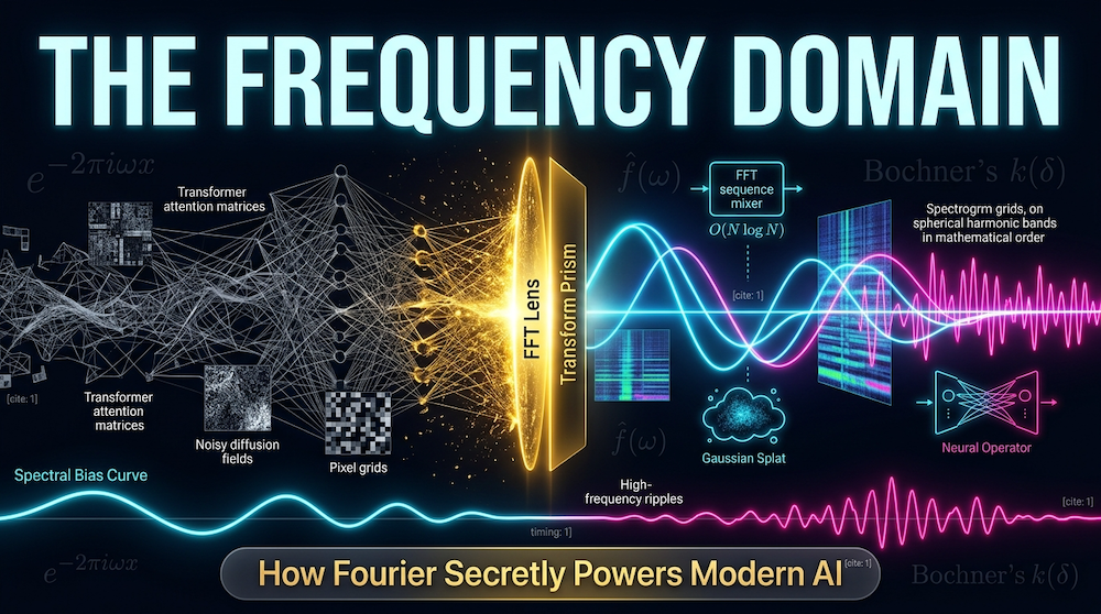
We have published twelve weeks of tutorials on what look like unrelated systems. We rendered 3D scenes from photographs. We asked what comes after the transformer. We rebuilt attention as a Gaussian process. We put uncertainty into world models, and then we made those world models plan. We treated training as a game with more than one player.
Each of those weeks stood on its own. This one does not. This piece is about a structure that was underneath all of them and that we mostly did not name at the time: the frequency domain.
That is a larger claim than it sounds, so let us be precise about what is being claimed and what is not. We are not claiming that every technique in modern AI is secretly a Fourier transform — that would be the kind of unfalsifiable tidiness that makes for a satisfying essay and bad engineering. We are claiming something narrower and more useful: that a specific, recurring difficulty — neural networks are bad at high frequencies, and the fixes look wildly different from each other — has one explanation, and that once you can see it, four or five techniques you already use stop being separate tricks and become instances of one method.
The method is old enough to be unglamorous:
Transform into a space where the hard operation becomes easy. Do the work there. Transform back.
Convolution becomes multiplication. A kernel becomes a probability distribution. A hard positional-encoding design problem becomes a question about which frequencies to sample. An mixing operation becomes . A differential equation becomes an algebraic one. In every case the win comes not from a better algorithm in the original domain but from a change of basis.
This piece is longer than our usual, for the same reason our game theory flagship was: the payoff is in the connections, and connections cannot be stated before their endpoints exist. We build the endpoints first.
A note on how to read the callbacks. When we point back at an earlier week, we link the published piece. If you have not read it, the callback is a bonus and not a prerequisite — every section here is self-contained. If you have, the callback is the point.
Companion notebooks:
00_fourier_features_from_scratch.ipynbbuilds random Fourier features from Bochner's theorem, verifies the approximation rate, and computes the neural tangent kernel before and after the feature map — measuring the claim in Section 3 rather than asserting it.01_fnet_vs_attention_vs_gpa.ipynbtrains dot-product attention, FNet and kernel-regression attention on one task with two independent bits, and measures the claims in Sections 5.2 and 5.3: FNet reads the global frequency bit perfectly with zero mixer parameters and the content-routing bit at chance, and the whole-block FFT speed-up runs about eight times below the FLOP-count prediction. Both are pure NumPy, CPU-only, with hand-derived gradients checked against finite differences, and both ship fully executed.
0. Changing the domain: a trick you already trust
Before any mathematics, we want to place the Fourier transform inside a family where you already trust the other members — because the move it makes is one that modern machine learning makes constantly, under different names: when data is hard to work with in the domain where it arrives, do not work harder there. Move it to a domain whose geometry matches the operation you need.
You use this trick every day.
Word embeddings. In their raw domain, words are discrete token IDs, and the question "are these two words similar?" is not merely hard — it is invisible. One-hot vectors are all equidistant from each other; the representation contains no notion of meaning at all. Map the tokens into a continuous vector space, and semantic similarity becomes geometry: a dot product, one instruction. Nothing was added to the data. The information was always there, distributed across co-occurrence statistics; the new domain is the one where it condenses into something a linear operation can read.
Vision–language encoders. Pixels and sentences have no common measure in their raw forms — there is no arithmetic that compares a JPEG to a caption. A CLIP-style dual encoder maps both into one shared space, and the incomparable becomes comparable: cross-modal similarity is again a dot product. Here the trick is used twice, on two domains at once, precisely so that the hard operation — "does this text describe this image?" — becomes the easy operation in the shared domain.
Kernel machines. The classical case, and the cleanest statement of the pattern. Data that no hyperplane can separate in its input space becomes linearly separable after a lift into a higher-dimensional feature space — and the kernel trick evaluates inner products in that space without ever visiting it. An SVM with an RBF kernel is not a cleverer linear classifier; it is an ordinary linear classifier operating in a domain chosen so that ordinary is enough.
The Fourier transform is this same move, with two specific differences that earn it a whole essay rather than a bullet in this list.
First, the target domain is not learned. An embedding space is fitted to a corpus; a kernel's feature space is chosen from a menu. Frequency space is given — fixed by mathematics, and (as Section 7 makes precise) determined by symmetry rather than by anyone's design choices. That is why the same construction reappears unchanged across signal processing, PDEs, and neural architectures across seventy years.
Second, the map is exactly invertible, and cheap in both directions. An embedding is lossy. A kernel lift is one-way — you compute inner products in the feature space but can never come back with a modified object. The FFT round-trips in with nothing lost. That is what lets the Fourier transform be used inside a computation — transform, operate, return — rather than only at the entrance to one, and it is the property the whole "transform, work, transform back" method of this article rests on.
So the honest answer to "is frequency just one more alternative domain?" is: yes — and it is not the only one. Wavelets are a domain (frequency, but localized — Section 8 says when you want them instead). The eigenbasis of a graph Laplacian is a domain (Section 7). The learned latent space of an autoencoder is a domain. The family is large, and choosing a member of it is the real design decision. Frequency is the member you reach for first when the operations you need are convolution, differentiation, or anything else that respects translation — because in the frequency domain, and only there, those operators become diagonal.
0.1 Why frequencies, specifically
There is a line widely attributed to Nikola Tesla: "If you want to find the secrets of the universe, think in terms of energy, frequency and vibration." We should be honest that no primary source for the quote has ever been produced — it is folklore, and we cite it as folklore, not scholarship. But folklore persists when it names something people keep experiencing, and what this line names is a real and repeatable experience: data that is an unreadable mess in the domain where it was recorded, and nearly crystalline one Fourier transform later.
Three examples, all of them boringly standard in their home fields, which is the point.
A piano chord. The recorded waveform of three notes played together is a tangled, aperiodic-looking squiggle; nothing about it announces "three notes." Its spectrum is a handful of sharp spikes — one family of peaks per note, at each note's fundamental and its harmonics. The question "which notes are being played?" is close to unanswerable by eye in the time domain and is read off in the frequency domain. Every guitar tuner exploits this.
A failing bearing. An accelerometer strapped to rotating machinery records what looks like noise. But a defect on a bearing race strikes the rolling elements at a characteristic rate fixed by the geometry, and in the spectrum that defect stands up as a clean peak at that frequency — visible weeks before the failure is audible. An entire industry of vibration-based condition monitoring consists, at its core, of reading spectra that say what time traces cannot.
Electricity demand. A months-long demand trace looks like weather-driven chaos. Its spectrum has unmistakable spikes at once per day, once per week, and once per year — the human rhythms that actually generate the signal. (EEG is the same story in another field: clinicians describe brain activity in frequency bands — alpha, beta, delta — because the raw trace resists the eye and the spectrum does not.)
Why does the world keep handing us signals with this property? Because so much measured data is generated by processes that oscillate, rotate, or repeat — resonating physical systems, spinning machines, planetary cycles imposing days and seasons. And there is a sharper version of that statement: for any linear, time-invariant process, complex sinusoids are the eigenfunctions — the inputs the system passes through changed only in amplitude and phase. For data generated by such processes, the frequency domain is not just a convenient rearrangement; it is aligned with the causes of the signal, which is why the structure looks like it snaps into focus. Where that generating story is absent — natural images at object scale, language — the raw Fourier domain loses much of its magic, and Section 8 draws that boundary honestly.
0.2 The transformer as the general case: learning the domain instead of choosing it
There is a stronger version of this section's argument, and it is worth stating carefully, because depending on how precisely it is phrased it is either the deepest idea in this article or an overreach.
The strong version goes: the transformer is the general case of "change the domain." Word embeddings choose one target space, for text. A CLIP-style encoder chooses one shared space, for images and captions. A kernel picks its feature space from a short menu. A transformer does not choose at all — it learns a very high-dimensional space, layer by layer, in which whatever structure matters for its training data becomes linearly accessible. On that reading the three examples above are not siblings of the transformer. They are special cases of it, distinguished mainly by having been discovered first.
A good deal of evidence points this way, and it is worth separating the parts that are solid from the part that is not.
The mechanism is already in the kernel family. Tsai et al. (arXiv:1908.11775) rewrite attention as kernel smoothing: each output is a kernel-weighted average of values, with the softmax acting as an (asymmetric, exponential) kernel. That is a rewriting rather than an analogy, and it means the transformer's core operation lives in the same family as Section 4's kernels — which Bochner's theorem will connect directly to the frequency domain. The bridge from this section to the rest of the article runs straight through attention itself.
The space really is shared across modalities. Perceiver (Jaegle et al., arXiv:2103.03206) was built as a modality-agnostic architecture: images, audio, point clouds and video enter the same latent space with almost no per-modality machinery — and, in a detail too apt to leave out, the structure it uses to tell positions apart is a bank of Fourier features. The most general learned-domain architecture of its generation reached for the given domain to encode position. Gato (Reed et al., arXiv:2205.06175) pushes the same idea further: text tokens, image patches, proprioceptive readings and motor actions are serialized into one sequence, one embedding space, one set of weights.
High dimension is what makes "concepts get distilled" more than a metaphor. The word2vec analogies (Mikolov et al., arXiv:1301.3781) were the first widely-seen demonstration that a learned space can put a relation into a direction. Toy Models of Superposition (Elhage et al., arXiv:2209.10652) supplies the capacity argument: a -dimensional space holds far more than nearly orthogonal directions, so a network can represent many more features than it has neurons by tolerating small interference. "A super-high-dimensional space in which concepts are distilled and structured" is not hand-waving — it is a statement with a Johnson–Lindenstrauss-flavoured bound behind it.
And the strongest form of the claim is contested, so we will not assert it. The Platonic Representation Hypothesis (Huh et al., arXiv:2405.07987) proposes that models trained on different modalities converge, as they scale, toward one shared statistical representation of reality. It is a genuinely interesting position paper. But a 2026 re-examination, Back into Plato's Cave (arXiv:2604.18572), reports that the evidence is fragile and regime-dependent: the alignment metrics degrade substantially as the evaluation set scales to millions of samples, and what survives looks like coarse semantic overlap rather than consistent fine-grained structure. Its summary — models trained on different modalities may learn equally rich representations of the world, just not the same one — is the version a practitioner should carry. Modality-shared, concept-structured spaces are real and useful. One universal space that all sufficiently large models converge on is not established, and the most recent measurement argues against it.
So here is the careful statement, the one we are willing to defend: the transformer is the most general member of the change-the-domain family that we know how to build, because it is the one that learns its domain rather than receiving it. And that is exactly the axis on which it trades against the Fourier transform:
| learned domain (transformer) | given domain (Fourier) | |
|---|---|---|
| what fixes the basis | data and gradient descent | symmetry |
| adaptivity | content-dependent | content-independent |
| invertibility | approximate at best | exact |
| cost to obtain | a training run | , and free |
| behaviour off-distribution | undefined | unchanged |
Neither column dominates. The left one can represent things the right one provably cannot; the right one is exact, cheap, and never has to be learned. Section 5.4 is what happens when people try to replace the left column with the right one, component by component — and it is the most direct answer this article has to the question of what a frequency-domain architecture would actually be.
With the family resemblance established, here is the transform itself.
1. The Fourier transform in sixty seconds
The one-sentence version: any reasonable signal can be written as a sum of sinusoids, and the list of how much of each sinusoid you need is as complete a description of the signal as the signal itself.
For a function on the real line, the Fourier transform and its inverse are
Four properties do all the work in this article.
Linearity. The transform of a sum is the sum of the transforms. Unexciting, and the reason everything downstream composes.
The convolution theorem. This is the load-bearing one:
Convolution — an operation involving every pair of positions — becomes pointwise multiplication, an operation, in frequency space. Since the FFT costs in each direction, you can convolve two length- signals in total by transforming, multiplying, and transforming back. Every "we replaced the quadratic thing with an FFT" architecture in Section 5 is this identity and nothing more.
Differentiation becomes multiplication. For a differentiable signal,
Differentiation — an operator that couples every point of a function to its infinitesimal neighbours — is, in frequency space, a pointwise multiplication by . Apply it twice and the Laplacian becomes multiplication by . The consequence is that a linear differential equation with constant coefficients, transformed, stops being a differential equation at all: it is an algebraic equation you can solve for by division. This identity is the engine of classical spectral PDE solvers, and Section 6.2 shows it resurfacing inside neural networks.
Parseval's theorem. Total energy is preserved: . The transform is a rotation, not a distortion. Nothing is lost, which is why "transform, work, transform back" is exact rather than approximate.
And one constraint that matters more in practice than its textbook prominence suggests. The uncertainty principle: a signal cannot be sharply localized in both position and frequency. Narrow in time means broad in frequency, and vice versa. This is not a quantum-mechanical fact that happens to have a signal-processing analogue; it is a theorem about Fourier pairs that quantum mechanics happens to inherit. It is also the reason the short-time Fourier transform and wavelets exist, and — as we will see in Section 3 — the reason you cannot simply demand that a network be accurate at all frequencies at once.
For discrete data we use the DFT, computed by the FFT in :
The FFT is arguably the most consequential algorithm of the twentieth century, and its speed is the reason the rest of this article is about engineering rather than about theory.
1.1 Two centuries of being under-rated, twice
It is worth pausing on how this piece of mathematics arrived, because the history is not the usual story of a tool being invented and then used. It is a story of a result being rejected, and then of the algorithm that makes it practical being discovered, written down, published, and ignored for a hundred and sixty years.
The transform was rejected by the best mathematicians alive. Joseph Fourier submitted his memoir on heat propagation in solids to the French Academy of Sciences in 1807. The committee included Lagrange and Laplace, and they did not approve it. The objection was the central claim: that an arbitrary function — including discontinuous ones — could be written as a sum of sines and cosines. Lagrange had taken a position against trigonometric series decades earlier, in the vibrating-string debates of the 1750s, and did not move. Fourier was not vindicated quickly; the Academy set heat conduction as its 1811 prize topic, he submitted an extended version, and he won in 1812 — with the referees' reservations about rigour attached to the award. The full treatment, Théorie analytique de la chaleur, appeared in 1822, fifteen years after the memoir the Academy would not accept.
And the referees were not being obtuse. Fourier's claim genuinely was not rigorous by the standards of 1807, and making it rigorous is one of the great projects of nineteenth-century mathematics: Dirichlet's convergence conditions, Riemann's integral (built, in part, to make sense of what a Fourier coefficient even is), Cantor's set theory (which grew out of the question of when a trigonometric representation is unique), and eventually Lebesgue's integral and the modern definition of a function. This is the concrete case for calling it one of the most important inventions in the history of mathematics, and it is stronger than "it turned out to be useful": the transform was too powerful for the foundations that existed, so the foundations had to be rebuilt around it. Most tools do not do that. Most tools are built on the foundations.
Then the algorithm was lost in plain sight. The divide-and-conquer trick that makes the discrete transform cost instead of is universally known as Cooley–Tukey, after the 1965 paper that set off digital signal processing. It was not new in 1965. Carl Friedrich Gauss had worked it out around 1805 — before Fourier's memoir — to interpolate the orbits of the asteroids Pallas and Juno from sampled observations. He wrote it in neo-Latin, never published it in his lifetime, and it appeared posthumously in his collected works, where it sat, available to anyone who cared to read it, until Heideman, Johnson and Burrus reconstructed the lineage in Gauss and the History of the Fast Fourier Transform (Archive for History of Exact Sciences 34(3), 1985).
That last episode is sometimes told as though a lost mathematics had been recovered. The documented version is less mystical and more useful: nothing was lost. Gauss's algorithm was correct, complete, and in print. What was missing was a machine fast enough for the constant factor to matter and an application that needed millions of transforms — and until those arrived, an optimal algorithm was a curiosity rather than an invention. The transferable lesson is that mathematics routinely runs a century or more ahead of the hardware that makes it consequential, which is worth remembering while reading the rest of this article: several of the architectures in Section 5 are limited today not by their mathematics but by which operations current accelerators happen to be good at (Section 5.3 puts numbers on that).
The reach of the thing, once the hardware caught up, is hard to overstate without sounding like a brochure, so here it is flatly: JPEG and MP3 are compression in the transform domain; MRI measures the Fourier transform of the body and inverts it to produce the image; X-ray crystallography reads molecular structure — including the structure of DNA — from diffraction patterns, which are Fourier transforms of the thing being imaged; radio astronomy synthesizes apertures the same way; Wi-Fi, 4G and 5G all run an inverse FFT in the transmitter and an FFT in the receiver, because OFDM is the convolution theorem sold as a modulation scheme. Ranking inventions is not a falsifiable exercise and we will not pretend otherwise. What is defensible is narrower and more striking: very few pieces of mathematics span that distance — from a rejected memoir about heat, to the foundations of analysis, to the radio in your pocket, to the mixing layer of a neural network.
1.2 Why audio got there first, and why vision did not
There is an asymmetry in that history which is easy to walk past and which turns out to explain most of Section 5.4. One modality moved into the frequency domain before digital computers existed and has never moved back out. The others did not follow, and the gap is measured in decades.
The audio chronology is worth laying out flatly, because the dates are the argument:
| Year | What happened |
|---|---|
| 1939 | Homer Dudley's vocoder analyzes speech into a bank of frequency-band energies and resynthesizes it; demonstrated publicly at the New York World's Fair |
| 1946 | Koenig, Dunn and Lacy's sound spectrograph (doi:10.1121/1.1916342) prints time–frequency energy on paper; Potter, Kopp and Green publish Visible Speech the following year |
| 1963 | Bogert, Healy and Tukey define the cepstrum — the spectrum of the log spectrum — to separate a signal from its echoes |
| 1965 | Cooley–Tukey. The FFT arrives after all of the above |
| 1971 | Atal and Hanauer's linear prediction (doi:10.1121/1.1912679) fits the vocal tract as an all-pole filter |
| 1980 | Davis and Mermelstein (doi:10.1109/TASSP.1980.1163420) show mel-frequency cepstral coefficients beat every competing representation. MFCCs become the front end for thirty years |
| 2012 | Hinton et al. (doi:10.1109/MSP.2012.2205597) replace the Gaussian mixture model with a deep network — on mel filterbank inputs. The neural network replaced the classifier, not the transform |
| 2022 | Whisper (arXiv:2212.04356) feeds a transformer an 80-channel log-mel spectrogram, 25 ms Hann window, 10 ms hop — the constants are in the released source |
Read the middle of that table again. The spectrogram predates the FFT by nineteen years — it was built from an analog filter bank and a rotating drum of heat-sensitive paper — and it predates deep learning by about sixty-five. The cepstrum was invented by one of the two authors of Cooley–Tukey, two years before the FFT paper, and not for speech at all: it came out of work on detecting the echoes in seismic recordings of nuclear tests. Audio arrived at the frequency domain from several directions at once and then simply stayed.
The vision equivalent — feeding a recognizer DCT or Fourier coefficients instead of pixels — is a 2018-and-later research topic that has not become anyone's default (Section 5.4's table). That is a seventy-year gap between two modalities that are both continuous, both sampled, both sensed by an organ. The board's question is the right one: if discreteness is what disqualifies text, what disqualified images?
Five things, and the first one does most of the work.
1. Speech has a linear, time-invariant generative process. Images do not. This is the real answer and everything else is detail. Speech is produced by a quasi-periodic glottal source passing through the vocal tract, which acts as a filter: the output is the convolution of source and filter. By the convolution theorem that is a product in frequency space, and taking a logarithm turns the product into a sum — at which point the two factors you actually care about, pitch and vowel identity, are additively separable by a linear operation. That is not an analogy for what MFCCs do; it is a line-by-line description of it, and the same statement covers room reverberation, which is convolution with an impulse response. The frequency domain does not merely represent speech compactly. It factorizes the physics that produced it.
Now try to write the corresponding sentence for a photograph. Image formation is projection and occlusion: a nearer object does not add to or convolve with the one behind it, it replaces it. Occlusion is not a linear time-invariant operator, so no change of basis diagonalizes it, and the Fourier transform has nothing to factorize. (Optical blur is a convolution, which is why deblurring has always been done with FFTs — but blur is the nuisance in an image, not the content. For speech, the convolution is the content.) This is Section 0.1's test applied honestly, and it is the same boundary Section 5.4 hits from the other side.
2. The ear is a spectrum analyzer; the eye is not. Von Békésy's Nobel-winning work established that the basilar membrane disperses frequencies along its length, so each hair cell responds maximally to its own band — the cochlea performs a physical, tonotopic spectral decomposition before a single neuron fires. The mel scale exists for the same reason: Stevens, Volkmann and Newman (doi:10.1121/1.1915893) measured perceived pitch in 1937, and a mel filterbank is a model of an organ. The retina has no comparable structure — it is spatially organized, and V1 simple cells behave like localized band-pass filters, which is a wavelet-like local analysis rather than a global transform.
That has a consequence people rarely state: vision never needed a hand-designed spectral front end because a convolution layer already is one. The Gabor-like filters that appear in a trained CNN's first layer are the local frequency analysis, learned. Audio's front end was engineered forty years before the learning machinery existed, so by the time neural networks arrived the spectrogram was already the interface and there was nothing to displace it. Vision's arrived in the opposite order. Some of the seventy-year gap is physics; some of it is which field got its answer before it had the option of learning one.
3. The spectrum is discriminative for speech, and much less so for images. Phoneme identity is the position of two or three spectral peaks — formants — which is why "Visible Speech" could be pitched as something a person might learn to read off a chart. Natural images, by contrast, nearly all share an approximately power spectrum (Field, doi:10.1364/JOSAA.4.002379), so the global magnitude spectrum is close to a universal constant across the dataset. Be careful here, because the strong form of this claim is false: Torralba and Oliva's Statistics of natural image categories showed spectral signatures do correlate with scene scale and with natural-versus-man-made, enough to support coarse "gist." But coarse gist is a different order of thing from the phoneme is right there in the picture.
4. Audio tolerates throwing away phase. Images do not. The entire mel-spectrogram pipeline discards phase, and Griffin–Lim (doi:10.1109/TASSP.1984.1164317) recovers something intelligible from magnitude alone — which is why magnitude-in, magnitude-out was a viable architecture for decades. Images run the other way: Oppenheim and Lim (doi:10.1109/PROC.1981.12022) showed that phase-only reconstructions stay recognizable while magnitude-only ones do not. So the cheap, real-valued version of "move to the frequency domain" — keep the magnitudes, drop the phases — is nearly free for audio and destructive for images. Destructive is worth scoping, because the absolute reading of it is false and bullet 3 above already said so: the magnitude spectrum alone still carries the coarse statistics Torralba and Oliva measured — scene scale, natural-versus-man-made — and magnitude-only descriptors have served texture and gist tasks on exactly that basis. What magnitude does not survive is anything depending on where the structure sits, which is most of recognition. There is no image Griffin–Lim. That is the same bullet as Section 5.4's complaint that FNet keeps only the real part of its DFT, arriving seventy years earlier and from the data side rather than the architecture side. A 2026 preprint, arXiv:2606.17037, reports the modern echo — transplanting Fourier phase between images moves the prediction of GFNet, ViT-B/16 and ResNet-50 with it, while removing image-specific magnitude barely dents accuracy — which we flag as recent and unreplicated, and which is not load-bearing here because the 1981 result already is.
5. Stationarity, dimension, and what a 1970s machine could do. The vocal tract reconfigures on a timescale of a few tens of milliseconds, so speech is quasi-stationary over a 20–30 ms window — which is the entire premise of the short-time Fourier transform, and why Whisper's window is still 25 ms. Images have no equivalent window: their statistics change discontinuously at every occlusion boundary, so a global 2D FFT deliberately mixes content across semantic boundaries. And the arithmetic mattered: a 256-point 1-D FFT at 8 kHz was real-time on 1970s hardware; a 2-D FFT over a megapixel was not.
And language. Text is disqualified before any of this. There is no sampling rate, no metric axis, and — decisively — word order carries syntax that is not shift-invariant, so translation invariance, the one thing a magnitude spectrum buys you for free, is the one property you must not have. That is why the text column in Section 5.4's audit is the empty one.
The honest caveat, which sharpens the rule rather than weakening it
Vision did adopt Fourier early and completely — just not for recognition. MRI measures k-space and inverts it; CT reconstructs through the projection-slice theorem; JPEG is a DCT codec; deconvolution is an FFT. And vision did try frequency for recognition: Fourier descriptors and Fourier-spectrum texture analysis were live research in the 1970s, and they lost to local gradient features like SIFT and HOG, because global spectra are wrecked by clutter and occlusion — reason (1) again, wearing different clothes.
So the predictor is not the modality, and it is not continuous-versus-discrete. MRI images are exactly as continuous as camera images and went Fourier immediately and totally. The rule that actually sorts the cases is this:
The frequency domain wins where the oscillatory structure is in the generating process or in the measuring instrument — not merely somewhere in the data.
Audio has both: the vocal tract generates it, the cochlea measures it. MRI has the instrument. Photographs have neither, and the transform is a change of coordinates with no physics behind it. Text has neither and no axis to put one on.
What this changes about Section 5.4
It supplies the missing why for a claim we made there — that the natural first modality for a frequency-native architecture is audio and robot action — and it adds one caution worth holding.
Eighty-three years is long enough for a convention to survive on inertia rather than merit, so the question is whether the mel filterbank is still right or merely entrenched. The head-to-head evidence says right. LEAF (arXiv:2101.08596) is a fully learnable drop-in replacement for mel filterbanks and reported beating them; the follow-up attempt to make it practical, EfficientLEAF (arXiv:2207.05508), is subtitled A Faster LEarnable Audio Frontend of Questionable Use and reports failing to show a clear advantage over fixed mel spectrograms. Meanwhile the models that abandon the front end entirely and consume raw waveform — wav2vec 2.0 (arXiv:2006.11477), WaveNet (arXiv:1609.03499) — learn band-pass filters in their early layers anyway.
Both outcomes point the same direction, and it is the direction Section 0.2 set up. Where the given basis is the one the learned basis converges to, the given basis is not a legacy convention; it is a solved problem, cached. That is a considerably stronger endorsement of the frequency domain for audio than eighty-three years of habit would be — and it is the cleanest available evidence that the "start with audio" advice at the end of Section 5.4 is not merely the path of least resistance.
Hold that claim at the strength its evidence supports, which is two head-to-head results and an observation about what waveform models learn in their first layers — not a theorem, and not a closed question. State the falsifier, as we do for the architecture case in Section 5.4: a learned front end that beats mel on a modern large-scale audio model and whose advantage survives an independent replication would overturn it. That is not a hypothetical bar. It is precisely the claim LEAF made and precisely the one the follow-up attempt failed to reproduce, which is why the cached-solution reading is the one the current evidence carries — and why it is the kind of claim that a single solid result could take back.
2. Spectral bias: the thing we kept running into and kept renaming
Here is the empirical fact that organizes this whole piece.
Neural networks trained by gradient descent learn low frequencies first, and high frequencies later — sometimes much later, sometimes never.
This is not a vague statement about "networks preferring smooth functions." It is measurable and it is sharp. Rahaman et al. (arXiv:1806.08734) fit ReLU networks to superpositions of sinusoids and tracked, frequency by frequency, when each component was learned. The low-frequency components are regressed first, regardless of their amplitudes; the high-frequency components lag far behind — and later work quantified the lag, with convergence time growing roughly as the square of the frequency. The same phenomenon has been studied under the name the Frequency Principle: during training, the error in the low-frequency band collapses long before the error in the high-frequency band moves at all.
The mechanism is not mysterious. Standard activation functions are piecewise smooth, and the Fourier spectrum of the function a network represents decays with frequency. Gradient descent moves fastest along directions where the loss is most sensitive, and for a smooth parameterization those directions correspond to the low-frequency content of the target. High-frequency error is real error, but it lives in a flat part of the landscape.
Two engineering consequences, pulling in opposite directions, and you have to know which one you are in.
When it helps. Spectral bias is a free regularizer. Noise in a dataset is typically broadband and disproportionately high-frequency; genuine structure is typically lower-frequency. A network that fits low frequencies first is a network that fits signal before noise. This is a large part of why early stopping works at all — you are stopping the model in the window where it has acquired the structure and not yet acquired the noise. It is also part of why heavily over-parameterized models generalize better than the classical bias–variance story predicts: the implicit bias of the optimizer, not the capacity of the model, is doing the regularizing.
When it hurts. When the thing you are trying to represent is high-frequency, spectral bias is not a helpful prior, it is the central obstacle. Sharp edges in an image. Fine geometric detail on a surface. Texture. A signal with genuine periodic structure at short wavelength. In those regimes a network will converge beautifully to a blurred version of your target and then sit there.
2.1 Where we already met this without naming it
When we built 3D Gaussian Splatting from scratch in W14, the optimization went through a distinct coarse-then-fine progression: a blurry blob resolving into structure, with fine detail arriving late and grudgingly. We explained the early behaviour in terms of gradient dilution — an MSE image loss is dominated, in raw magnitude, by the many low-detail background pixels rather than by the few high-detail ones.
That explanation was right, and it was half the story. Gradient dilution is itself a spectral statement. "Most of the loss mass lives in the smooth background" and "most of the loss mass lives at low spatial frequency" are the same sentence in two vocabularies. The coarse-to-fine trajectory we watched was the Frequency Principle rendering itself in front of us.
The W16 work on 4D Gaussians added a second axis and the same pattern appeared along it. Slow motion in a dynamic scene — a camera drifting, a body swaying — is low temporal frequency and is captured early. Fast motion is high temporal frequency and is captured late or smeared. And the sampling constraint that governs whether it can be captured at all is Nyquist: a deformation field reconstructed from frames at a given rate cannot represent motion faster than half that rate. The failure mode we described as "fast motion is hard" has an exact quantitative form.
2.2 Diffusion is spectral bias, deliberately reversed
The most striking instance is one where the field built its schedule around the phenomenon without always framing it that way.
In our W29 probabilistic 3D week we treated diffusion models as reconstruction under uncertainty. Look at what the denoising trajectory does in frequency space. Adding isotropic Gaussian noise raises the noise floor uniformly across all frequencies. But natural images have power spectra that fall off roughly as a power law — most of their energy is at low frequency. So as noise accumulates, the high-frequency content of the image drops below the noise floor first, and the low-frequency content survives longest.
Run that backwards, which is what sampling does, and the model necessarily recovers low frequencies first and high frequencies last. That is why early denoising steps fix global composition and late steps fix texture and edges. A diffusion schedule is, read spectrally, a frequency curriculum: a prescription for which band of the spectrum the model is responsible for at which step.
So spectral bias and diffusion are not merely analogous. Spectral bias is the direction gradient descent goes on its own; a diffusion schedule is that same ordering imposed deliberately and run in reverse.
2.3 Measuring it, rather than believing us
Everything above is checkable on your own model in about ten minutes, and we would rather you check it than take it on faith. The diagnostic is short enough to state in full.
Take your model's predictions and the ground truth on a held-out set. Compute the radially averaged power spectrum of each: FFT the 2D field, take the squared magnitude, and average over annuli of constant radius in frequency space, so that each bin corresponds to a spatial frequency band regardless of orientation. Plot the two curves on log axes, and plot their ratio.
What you are looking for is the frequency at which the prediction curve falls away from the target curve. That crossover is your model's effective bandwidth, and it is a far more actionable number than a validation loss. A model whose curves track to the Nyquist limit and then diverge is doing as well as the data allows. A model whose curves diverge at a quarter of Nyquist is leaving detail on the table that is present in the data, and further training at that configuration will close the gap only at the crawl spectral bias dictates — the checkpoint plot below is what distinguishes slow from stalled, and either way the economical fix is in the representation, not in more optimization.
Do the same thing over training checkpoints and you can watch the Frequency Principle happen: the crossover point marches outward as training proceeds, quickly at first and then barely at all. The epoch at which it stops moving is a principled place to consider early stopping, and it is visible in this plot long before validation loss flattens convincingly.
This is also the cheapest way to distinguish two failure modes that look identical in aggregate error. Underfitting high frequencies shows up as a prediction spectrum that decays too fast. Hallucinating high frequencies — a model inventing texture that is not in the data, which is what happens when you over-scale the Fourier features from the next section — shows up as a prediction spectrum with more energy than the target at high frequency. Both can produce the same MSE. They demand opposite fixes, and a scalar loss cannot tell you which one you are looking at.
3. Fourier features: buying high frequencies back
If the problem is that networks cannot easily represent high frequencies, the fix is to stop asking them to. Put the high frequencies in the input.
Given an input , instead of feeding to the network, feed
where is a matrix of frequencies — either a fixed geometric ladder or drawn from some distribution. The network now sees coordinates that already oscillate rapidly. Representing a high-frequency function of becomes a low-frequency function of , which is exactly the regime gradient descent is good at.
This is the single most reused trick in the last six years of neural rendering, and it is usually introduced as an implementation detail. It is not. Tancik et al. (arXiv:2006.10739) gave the explanation, and the explanation is the interesting part.
Analyze the network through its neural tangent kernel. A plain coordinate MLP has an NTK that is effectively a narrow, non-stationary kernel: how strongly two inputs influence each other depends on where they are, not just how far apart they are. Compose the network with a Fourier feature map and the NTK becomes stationary — a function of alone — and, crucially, its bandwidth becomes a quantity you choose by choosing the distribution of .
That reframes positional encoding completely. It is not a formatting convention for coordinates. It is kernel design: you are specifying the spatial frequency content your model is able to fit, before training starts. Pick with too little spread and you get the blurry underfit the plain MLP would have given you. Pick it with too much and you get high-frequency noise and overfitting — the network can now represent garbage at the sampling scale, and it will. The scale of is a genuine hyperparameter with a genuine optimum, and Tancik et al.'s central experiment is a sweep showing exactly that U-shaped curve.
3.1 The W14 callback, now with the mechanism attached
NeRF's positional encoding — the ladder at geometrically spaced frequencies that everyone copies — is precisely this construction. When we covered Marble-like architectures and image-to-3D in W14, the encoding was in the pipeline as a given. The reason it is there: without it, a coordinate MLP asked to output radiance at a point produces a soft, low-detail field, because it is being asked to learn a high-frequency function of raw coordinates and spectral bias forbids it.
There is a second Fourier structure hiding in the same week that is easy to miss. 3D Gaussian Splatting represents view-dependent colour with spherical harmonics. Spherical harmonics are the Fourier basis on the sphere — the eigenfunctions of the Laplacian on , exactly as complex exponentials are the eigenfunctions of the Laplacian on the line. The SH degree you pick is a bandwidth choice: degree 0 is a constant colour with no view dependence, higher degrees buy you sharper specular variation. Every 3DGS implementation is doing a truncated Fourier expansion in the angular variable and calling it a colour model.
So W14 used Fourier structure twice, in two different variables, and we discussed neither as such at the time.
3.2 The practitioner's version
Strip the theory and this is a short, usable rule.
- If your model outputs a smooth field over a continuous domain — coordinates, time, angles — and the output is blurrier than the data, the first thing to try is a Fourier feature map on the input.
- The frequency scale is the hyperparameter that matters, more than width or depth. Sweep it. The optimum is a genuine interior optimum.
- Match the bandwidth to the sampling rate of your data. Encoding frequencies above the Nyquist limit of your observations lets the model invent detail that nothing in the data constrains, which is aliasing with extra steps.
- If detail appears too slowly, consider increasing the bandwidth over training rather than fixing it — a progressive frequency curriculum, which is the same shape as the diffusion schedule from Section 2.2 and works for the same reason.
3.3 The failure mode on the other side: aliasing
Section 3.2 says "match the bandwidth to your sampling rate" in one line. That line deserves more, because violating it produces an artifact that practitioners routinely misdiagnose as a training problem.
If you encode frequencies above what your observations can constrain, the model acquires the capacity to represent detail at that scale without acquiring any information about it. The optimizer will happily use that capacity: it will fit high-frequency structure that explains the training views and corresponds to nothing in the scene. In a neural renderer this shows up as shimmering and crawling texture when the camera moves, or detail that changes character with viewing distance. It looks like instability. It is aliasing — the model representing frequencies above the Nyquist rate of its data, exactly as a texture sampled without filtering does.
The clue that distinguishes it from ordinary overfitting is scale dependence. Ordinary overfitting degrades held-out performance uniformly. Aliasing from over-wide Fourier features degrades it as a function of resolution or distance: render the same scene closer and it is fine, render it further and it breaks up, because at the further distance each output pixel integrates over a region containing several periods of the encoded frequency.
That observation is also the fix, and it is the insight behind the anti-aliased variants of coordinate networks. Instead of encoding a point, encode the region that the point's pixel actually covers — a cone or a volume — by integrating the Fourier features over that region. Integrating over a region of width attenuates the result by roughly (with ; the exact constant depends on the region's shape, and it is the decaying envelope that matters), which drives high-frequency components toward zero automatically whenever the sampling region is wide relative to their period. The encoding becomes scale-aware: the same query returns a sharp encoding when observed closely and a smoothed one when observed from far away, with no hand-tuned level-of-detail heuristic.
The general principle survives outside rendering. Fourier features encode an assumption about sampling density, and if that density varies across your domain, a single fixed bandwidth is wrong somewhere. Either make the encoding adaptive, or restrict the bandwidth to what the sparsest region of your data supports and accept the loss of detail in the dense regions.
4. Bochner's theorem: kernels and spectra are the same object
Section 3 said "Fourier features make the NTK stationary and let you choose its bandwidth." The theorem that licenses that sentence is worth stating properly, because it is the bridge between two of our weeks and because it is the most underrated result in this article.
Bochner's theorem. A continuous, shift-invariant kernel is positive definite if and only if it is the Fourier transform of a non-negative finite measure:
Read it slowly, because the content is not the formula. It says that every stationary kernel is a probability distribution over frequencies, and every distribution over frequencies is a kernel. The two objects are not analogous, not related, not dual in some loose sense. They are the same mathematical object in two coordinate systems.
Concretely:
| Kernel | Spectral density |
|---|---|
| RBF / squared exponential | Gaussian |
| Matérn | Student- |
| Laplacian | Cauchy |
| Periodic | Discrete spikes at harmonics |
"The RBF kernel is smooth" and "the RBF kernel's spectral density is Gaussian, so it has essentially no mass at high frequency" are the same statement. The reason a GP with an RBF kernel cannot fit a rough function is not a fact about GPs; it is a fact about where that Gaussian puts its mass.
4.1 Random Fourier features, and why they follow immediately
Bochner's theorem is also an algorithm, which is Rahimi and Recht's 2007 observation. If is the Fourier transform of a probability measure , then
and any expectation can be approximated by sampling. Draw , define , and then
An infinite-dimensional kernel becomes an explicit -dimensional feature map, computed by sampling frequencies from the kernel's own spectrum. Kernel ridge regression drops from to ; GP inference becomes tractable on data sizes where the exact cubic method is hopeless.
Now notice what is. It is a Fourier feature map — the same from Section 3. Positional encoding in a neural renderer and kernel approximation in a Gaussian process are literally the same construction. The difference is only in where comes from: sampled from a kernel's spectral density in one case, chosen as a geometric ladder in the other. This is why Tancik et al.'s NTK result works out so cleanly — composing with is choosing a stationary kernel by specifying its spectrum.
4.2 The W28 callback: attention's chain has one more link than we showed
In W28 we argued that attention is a kernel: softmax attention is Nadaraya–Watson kernel regression with an exponential-inner-product kernel, queries are test points, keys and values are training data, and the GP treatment follows from there. That week ended at the kernel.
The chain does not end at the kernel. It continues:
Two consequences that are practical rather than decorative.
First, the efficient-attention literature is a random-features literature in disguise. Performer-style linear attention approximates the softmax kernel with a sampled feature map so that attention factorizes into two linear passes — the Rahimi–Recht move of Section 4.1, with one honest wrinkle. is not shift-invariant, so Bochner does not apply to it directly; the construction routes through a Gaussian-kernel factorization, and Performer's estimator uses positive random features rather than the trigonometric ones, precisely because the trigonometric estimator's variance explodes where the softmax kernel is near zero — which is most of a long attention row. The spirit is Section 4.1 — approximate a kernel by sampling its feature expansion, with accuracy governed by how many features you draw; the letter needed new engineering, and the difference is a good example of why "the same idea" still earns its own paper.
Second, attention has a bandwidth, and you can reason about it. The temperature of the softmax sets how quickly similarity decays with distance in embedding space, which by Bochner is a statement about how much high-frequency mass the induced kernel carries. Sharp attention is a wide-band kernel: expressive, and able to represent abrupt changes in what a token attends to. Diffuse attention is narrow-band: smooth, stable, and unable to make sharp distinctions. The familiar advice to scale by is bandwidth control.
4.3 Spectral mixture kernels: designing in the domain where design is easy
The payoff of "kernels are distributions over frequencies" is that you can design in whichever of the two domains is easier, and for structured data the spectral domain is much easier.
Suppose your data has periodic structure and you do not know the period. In kernel space you would need to guess a functional form. In spectral space the question is trivially posed: put a mixture of Gaussians over and learn the mixture. Each component's mean is a frequency the model has discovered — its reciprocal, the period; its variance is how strictly periodic that component is; its weight is how much of the signal it explains. Inverse-transform the mixture and you have a valid stationary kernel — positive-definiteness is free, courtesy of Bochner. This is Wilson and Adams' spectral mixture kernel, and it can extrapolate periodic structure rather than merely interpolate it, which ordinary RBF-kernel GPs conspicuously cannot.
This connects directly to W33's planning under uncertainty. A planner that models environment dynamics with a GP and an RBF kernel has assumed, without being asked, that the dynamics are smooth and aperiodic. For an environment with genuine cycles — day/night, traffic, seasonality, any rhythm at all — that assumption does not merely add error, it removes the model's ability to extrapolate the one structure most worth extrapolating. A spectral mixture kernel fixes it, and the fix is a modelling decision made entirely in frequency space.
5. Fourier as architecture: when the FFT replaces the mixing layer
So far the Fourier transform has been an analytical lens. Now it becomes a layer.
Self-attention costs in sequence length because every token is compared with every other. The convolution theorem offers a different way to make every position depend on every other position: transform, multiply, transform back, in .
FNet (Lee-Thorp et al., arXiv:2105.03824) takes the most aggressive version of this. Replace the entire self-attention sublayer with an unparameterized 2D DFT over the sequence and hidden dimensions, and keep only the real part. No learnable parameters in the mixing operation at all. The reported result is the interesting one: roughly 92–97% of BERT's accuracy on GLUE while training about 1.7–1.8× faster at standard 512-token lengths (80% faster on GPUs, 70% on TPUs, by the paper's own numbers), with the speed gap widening substantially in FNet's favour as sequences get longer.
The lesson is not "attention is unnecessary." It is sharper and more useful: a large fraction of what a mixing layer needs to do is simply "let every position see every other position," and that is a fixed, content-independent operation that costs . Attention's learnable, content-dependent routing is worth real accuracy — but it is a smaller fraction of the total than the architecture's prominence suggests. FNet measures the size of that fraction, which is why it is a better paper than its accuracy numbers imply.
GFNet (Rao et al., arXiv:2107.00645) takes the moderate version: FFT into frequency space, multiply by a learnable global filter, inverse FFT. By the convolution theorem this is a global convolution with a learned kernel the size of the whole image, at . You keep learnability and still avoid the quadratic cost. The learned filters are also directly interpretable — you can look at which frequency bands a layer has decided to amplify or suppress.
5.1 The W15 callback: we asked the right question and had half the answer
In W15 we asked what comes after the transformer and surveyed the alternatives. Re-read that list spectrally and it is much less of a list.
State-space models are frequency filters. A linear time-invariant system is defined by its frequency response. S4 and its descendants apply a long convolution whose kernel is parameterized by a state-space matrix, and the convolution is computed via FFT precisely because of the convolution theorem. The HiPPO initialization that makes S4 work is a choice about which frequencies the state retains. Mamba's selective scan makes the parameters input-dependent, which breaks strict time-invariance — so Mamba is not a fixed filter — but the right way to describe what selectivity buys is an adaptive spectral filter: a system that changes its frequency response based on what it is currently reading.
Hyena is the most explicit case. It replaces attention with implicit long convolutions, parameterized by a small network that generates the kernel, and evaluated by FFT. The subquadratic scaling is the convolution theorem, stated as an architecture.
So the honest summary of W15 is this: the leading families of post-transformer architecture are, with few exceptions, ways of doing global mixing in frequency space. They differ in how much of the filter is learned, and whether it adapts to the input. That is a much more navigable map than a list of unrelated names, and it tells you what question to ask about the next architecture that appears.
5.2 A caution against over-reading this section
A synthesis piece should be honest about where its lens stops working, so: the FFT mixing story is not a claim that attention is obsolete, and the benchmarks do not support that claim. FNet loses accuracy. GFNet is strongest in vision, where translation-invariance-flavoured priors fit the data. The fixed, content-independent character of an FFT is exactly what makes it cheap and exactly what makes it weaker at tasks requiring sharp, input-dependent routing — retrieval, copying, precise long-range reference. Mamba's selectivity exists because the non-adaptive version was not sufficient.
What the frequency view gives you is not a winner. It is the right axis to compare on: how much of your mixing is fixed versus learned, global versus local, content-independent versus adaptive. The best architectures in 2026 are mixed — cheap spectral mixing in most layers, expensive attention where routing genuinely matters. Knowing the axis is what lets you make that trade deliberately.
5.3 Where the crossover actually is
" beats " is true asymptotically and frequently irrelevant in practice, so it is worth being concrete about when the spectral route pays.
Compare the operation counts directly. Attention over a sequence of length with model dimension costs on the order of for the score matrix and the same again for the weighted sum. An FFT-based mixer costs on the order of . The ratio is therefore roughly — which at is about 57, at is about 341, and at is about 4,100.
Those ratios look decisive and they overstate the practical gain substantially, for three reasons worth knowing before you rewrite a model.
Attention is not where all the time goes. In a standard transformer block the position-wise feed-forward network carries a large share of the FLOPs, typically the majority at short sequence lengths. Removing the entire attention cost cannot speed up the block by more than the fraction attention accounted for in the first place — the usual ceiling that applies whenever you optimize one component of a pipeline.
Attention is extremely well optimized and the FFT is not, on this hardware. Dense matrix multiplication maps onto tensor cores at near-peak throughput. FFTs are memory-bandwidth-bound, with strided access patterns that use a fraction of available FLOPs. A theoretical advantage of 50× can easily shrink to a wall-clock advantage of low single digits, or vanish. Measure; do not infer from the exponent.
The relevant scaling is memory, not compute. The reason quadratic attention actually hurts in production is usually the score matrix, which at long context dominates memory and bandwidth. Approaches that avoid materializing it — FFT mixing among them — win on the resource that binds first, and this is a better argument for them than the FLOP count is.
The honest summary: below roughly a thousand tokens the spectral route is rarely worth it; in the tens of thousands it is clearly worth evaluating; and the decisive variable is memory pressure rather than arithmetic. This is also why the FNet results widen in FNet's favour with sequence length — the published comparison is measuring the crossover, not a fixed advantage.
5.4 Has anyone rebuilt the transformer in frequency space?
Section 0.2 set up a trade between a learned domain and a given one. Sections 2 through 5 have now shown the given one turning up inside positional encodings, kernels, mixing layers and state-space models. The obvious question follows: what if you took the transformer apart and moved every component into the frequency domain — the token embedding, the positional embedding, the multimodal embedding, the action embedding, the mixing layer, the output head — rather than swapping one part at a time?
We went looking for the work. The answer is more interesting than yes or no: almost every component has been done, mostly outside language and mostly at small scale; the end-to-end version has not; and the reason it has not is specific and mathematical rather than an oversight.
The audit
| Component | Frequency-domain version | State of the art |
|---|---|---|
| Positional embedding | Sinusoidal PE; RoPE (arXiv:2104.09864); FoPE (arXiv:2412.17739) | Done, shipped, and winning — the frontier default is already a frequency-domain component |
| Attention itself | Performer (arXiv:2009.14794), Random Feature Attention (arXiv:2103.02143) — Bochner random features for the softmax kernel | Deployed; you may be running it without calling it spectral |
| Token mixing | FNet, GFNet, AFNO (arXiv:2111.13587), SpectFormer (arXiv:2304.06446), SVT (arXiv:2311.01310) | Most developed branch. Hybrids win; pure spectral loses (numbers below) |
| Sequence compression | Fourier Transformer (arXiv:2305.15099) — DCT to strip redundancy from hidden sequences | Works, narrow adoption |
| Token / word embedding | Complex-valued embeddings as continuous functions of position (arXiv:1912.12333); Wave Network (arXiv:2411.02674) | The thinnest column. Small models only; nothing at scale |
| Multimodal embedding | Audio: STFT / mel front ends, universal for decades. Vision: DCT-domain inputs (arXiv:2002.12416). Text: — | Already asymmetric: one modality done long ago, one partial, one with no natural definition |
| Action embedding | FAST (arXiv:2501.09747) — DCT + BPE over action chunks | The strongest single result, and already being displaced (below) |
| Output head | Fourier Head (arXiv:2410.22269) — a learned Fourier series in place of softmax-over-bins | Works where the target is a smooth continuous quantity |
| The whole stack, end to end, causal, at language scale | — | Nobody has built it |
There are now enough attempts in the vision branch alone to require a survey — Aslan et al., Frequency-Domain Vision Transformers: Architectures, Applications, and Open Challenges (Applied Sciences, doi:10.3390/app16042024) — which is itself part of the answer to "has anyone tried": many people have, and overwhelmingly not on text.
Three findings come out of that table.
Finding 1: the positional embedding was frequency-domain from the start, and it is the component that improved most
This one is easy to miss because of how normal it has become. The original sinusoidal positional encoding is a Fourier feature bank, chosen deliberately so that a relative shift would be a linear function of the encoding. One component of the 2017 transformer was designed in frequency-domain terms, and it is the component that has survived every redesign since.
RoPE (Su et al., arXiv:2104.09864) made it sharper — position becomes a rotation by an angle proportional to position times a per-dimension frequency — and it is now the default in essentially every open frontier model. FoPE (arXiv:2412.17739) then made the identification exact: analysed with discrete-signal-processing tools, RoPE is implicitly computing a non-uniform discrete Fourier transform, and the periodic extension that lets a model read past its trained context is degraded by what the authors call spectral damage — contributed by the linear layers and activation functions outside attention, and by under-trained frequency components arising from time-domain truncation. Their fix is to model each dimension as a Fourier series — a dominant frequency plus harmonics — and zero out the destructive components; they report more stable perplexity and more consistent needle-in-a-haystack accuracy across context windows than RoPE or ALiBi.
That result deserves more attention than it received, because of what it says about the architecture around it: the one frequency-domain component we already ship is being damaged by the time-domain components surrounding it. Hold on to that; it is the strongest argument in this section for the research direction at the end of it.
There is a companion result that is even harder to un-see. Barbero et al. (arXiv:2410.06205) examined how a trained model actually uses RoPE's frequency bands, and found that Gemma 7B exploits the highest frequencies to build robust positional attention patterns, while greatly preferring the lowest frequencies to carry what the authors suspect is semantic information. Nobody specified that allocation. The model discovered a frequency budget, and split it between position and meaning.
Finding 2: everything else has been tried — mostly in vision, robotics and audio, almost never in language
Token mixing is Section 5's material and the deepest branch. Attention itself has a frequency-domain formulation already in production: Performer and Random Feature Attention approximate the softmax kernel with random Fourier features, which is Section 4's Bochner construction cashed in as an efficiency technique. Spectral attention is not a speculative idea; it is a shipped one.
Multimodal embedding is already asymmetric, and almost nobody says so out loud. Audio moved to the frequency domain before deep learning existed — STFT and mel spectrograms are the input to effectively every speech model, so for one modality the migration finished decades ago and was never reversed. Section 1.2 works through why the asymmetry exists, and the short version matters for this audit: audio's generating process and its sensing organ are both spectral, and vision's are neither. Vision has a partial version: Xu et al. (arXiv:2002.12416) feed DCT coefficients directly out of the JPEG pipeline, discarding high-frequency channels, and DCT-domain transformers exist for compressed-domain tasks. Text has nothing comparable. So the honest status of "a unified multimodal frequency embedding" is: it already exists for one modality, was tried and not adopted for another, and has no agreed definition for the third.
Action embedding produced the strongest result in the whole audit, and then the most instructive one. FAST (Pertsch et al., arXiv:2501.09747) — the name stands for Frequency-space Action Sequence Tokenization — normalizes action chunks by quantiles, applies a DCT per action dimension, quantizes the coefficients, and BPE-compresses the result. It exists because the obvious scheme, per-timestep per-dimension binning, fails outright on dexterous high-frequency robot data. Paired with the π0 VLA it matched diffusion-based policies while cutting training time by up to 5×, and FAST+ ships as a black-box tokenizer trained on a million trajectories. If you want one clean demonstration that moving an embedding into the frequency domain can rescue a problem rather than merely accelerate it, this is it.
Now read the sequel. FASTer (arXiv:2512.04952) replaces the DCT stage with a learned vector-quantized tokenizer over action chunks and reports better reconstruction quality, higher token utilization, and stronger cross-task and cross-embodiment generalization. That result is recent and not yet independently replicated, which is the appropriate weight to give it. That is the left-hand column of Section 0.2's table overtaking the right-hand column, on the one problem where the right-hand column had just won decisively. Both halves are the finding. The given basis was what made the problem tractable at all; a learned basis fitted to the data then passed it. Expect that shape to recur — and notice that it is an argument about maturity, not about correctness: a fixed basis wins when data is scarce and structure is known, and a learned one wins when data is abundant.
Finding 3: nobody has built the whole stack, and the reason is a theorem
The natural suspicion when a promising idea keeps under-performing is that either the surrounding design is inadequate or the idea was never what the architecture was built for. For this question, neither is right. There is a third answer, and it is measurable.
FNet's own paper contains the number that settles it. Beyond the headline that FNet reaches 92–97% of BERT on GLUE, the authors report:
"We find that FNet hybrid models containing only two self-attention sublayers achieve 97 − 99% of their BERT counterparts' accuracy on GLUE, while still running 40 − 70% faster."
and they specify the placement: the final two Fourier sublayers are the ones replaced, because replacing the last layers worked best. Read that as a measurement rather than a benchmark result. Ten of twelve layers do not need content-dependent routing. Two do, they are the last two, and they are not optional. That is neither "spectral mixing doesn't work" nor "attention is unnecessary" — it is a quantification of how much of a language model's work is genuinely content-dependent, and the answer is: a small fraction, concentrated late, and indispensable.
Why it must come out that way follows from the test in Section 8.1. The Fourier basis is the eigenbasis of translation. It diagonalizes exactly those operators that commute with shifts. A layer whose job is to decide based on what the tokens are — resolve this pronoun, retrieve that name, copy this span — is by construction not shift-invariant, so no fixed spectral filter can diagonalize it. The ceiling is a theorem, not a shortfall of engineering effort. It is also the same boundary Section 0.1 drew when it said the frequency domain loses its magic where the generating process does not oscillate, and the same one Section 8 draws for non-stationary data. Language is on the wrong side of both lines.
Four further obstacles are engineering rather than mathematics. They matter because they are what a serious research programme would actually have to beat.
Causality. FFT-based convolution is inherently non-causal: the transform sees the whole sequence. Decoder-only language models need a strict causal mask. Making spectral mixing causal costs you either chunking — which surrenders the global-mixing win — or the machinery that state-space models already use. This is very likely why the frequency-domain successes in language arrived dressed as SSMs (Section 5.1) rather than as an explicit FFT layer.
Nonlinearity forces a round trip. The entire advantage is that shift-invariant linear operators are diagonal in frequency. GELU, softmax and LayerNorm are not. So a "frequency-domain transformer" transforms back every block and pays two FFTs per layer, and the savings shrink with depth. FoPE's spectral damage is precisely this bill, observed empirically: it is the interfaces between frequency-domain and time-domain components that leak.
Phase carries the information, and half the literature discards it. FNet keeps only the real part of its DFT. Real-valued spectral mixing constrains the implied phase to , and you cannot express a content-dependent shift with two phases. Complex-valued deep learning is also badly served by current kernels, quantization tooling and mixed-precision paths — so the implementation that is cheap to write is the one that throws away the quantity the approach depends on.
And: what is "frequency", over a vocabulary? Along the sequence axis frequency has a clear meaning — how fast a feature varies with position. Along the embedding axis it does not: FNet's second DFT runs over hidden dimensions whose ordering is arbitrary, so the "spectrum" it computes has no semantic referent. It functions as a mixing operation; it is not a spectral analysis of anything. A frequency-native text embedding has to answer what oscillates, and nobody has a satisfying answer. Audio does (pressure, over time). Video does. Robot actions do (joint angles, over time) — which is exactly why FAST works and why the thin column in the table is the text one.
The two approaches, side by side
If you are weighing whether to put engineering into this, the comparison is worth stating plainly:
| Frequency-native | Time/token-domain (status quo) | |
|---|---|---|
| Cost | , and no score matrix to materialize — the resource that binds first (Section 5.3) | compute and memory, mitigated by FlashAttention-style tiling |
| Exactness | Parseval: the transform is a rotation; nothing is lost per round trip | Every learned projection is lossy |
| Parameter efficiency | One complex scalar per frequency buys a global receptive field (GFNet) | Global reach costs a full attention block |
| Spectral bias | Explicitly controllable — you choose the bandwidth (Sections 2–3) | Inherited and fought; attention is itself a low-pass filter (arXiv:2203.05962), which is why deep ViTs oversmooth |
| Length / resolution | Defined on continuous frequency, so it extrapolates by construction (FNO discretization invariance; FoPE's length generalization) | Extrapolation is an open research area with a literature of patches |
| Interpretability | Learned filters are readable band by band | Attention maps are suggestive and contested |
| Content-dependent routing | Cannot express it — a fixed basis is content-independent by definition | Its whole purpose; the measured 97–99% gap is exactly this |
| Non-stationary data | A global basis over a signal whose statistics drift; needs STFT or wavelets, losing the clean theory | Handles it natively — attention is local and global at once |
| Causal decoding | Structurally awkward; non-causal by default | Native |
| Discrete symbols | No natural frequency axis over a vocabulary | Native |
| Hardware | FFTs are bandwidth-bound and use a fraction of peak FLOPs | Dense matmul runs at near-peak on tensor cores |
| Ecosystem | Thin: weak complex-number support, few quantized kernels, little serving infrastructure | A decade of kernels, quantization, and serving stacks |
The pattern in that table is not "one of these is better." It is that the two columns have complementary failure modes, which is precisely why the empirical winners are hybrids: cheap spectral mixing in most layers, expensive content-dependent routing where routing actually happens.
The case for a frequency-native transformer, and the experiment that would kill it
So: is there a research direction here, or is the hybrid the end of the story? We think there is a direction, and the strongest argument for it is not the speed one — Section 5.3 explains why FLOP-count arguments oversell.
The strongest argument is FoPE's: the damage is at the interfaces. Every attempt in the audit is a frequency-domain component dropped into a time-domain stack, so every one pays a conversion at both ends — and FoPE demonstrated that the conversion is lossy in a way you can measure, and that it costs length generalization specifically. That observation motivates exactly one hypothesis: remove the interfaces rather than improve the components. A frequency-native architecture is what that would look like.
Concretely, such a thing would need five parts, in rough order of difficulty:
- A complex-valued residual stream that preserves phase end to end, rather than taking the real part at each block.
- A causal spectral mixer — the genuinely hard one, and the reason this has not been done at language scale.
- A nonlinearity that means something in frequency space, or an explicit, budgeted policy for how often the stack round-trips.
- A defensible frequency axis for discrete tokens — most plausibly by abandoning the idea of a per-token spectrum and defining frequency only along the sequence axis.
- An output head in the same basis. Fourier Head is a working starting point.
Parts of (1) and (2) are being probed right now. FourierQK (arXiv:2607.07478) reports that FFT-based spectral preprocessing of the query and key projections improves language modelling even with random, unlearned filters — if that holds up under replication, it is a strong hint that the time-domain stack leaves spectral structure unused. FourierMoE (arXiv:2604.01762) routes tokens to experts specialized by frequency band and reports that different layers of an LLM have heterogeneous frequency sensitivity. Neither is a frequency-native architecture. Both are evidence that the interfaces are where the unclaimed value sits. We flag them as recent and not yet replicated, which is the appropriate weight to give a 2026 preprint.
And because a research direction without a falsifier is an enthusiasm, here is the experiment we would run first, before building anything: hold parameters, training data and achieved hardware utilization fixed, and ask whether a complex-valued, phase-preserving stack beats an equal-FLOP real-valued one at the same context length. If the advantage disappears once utilization is controlled — and Section 5.3 gives every reason to expect wall-clock advantages to evaporate on tensor-core hardware — then the interfaces were not the bottleneck, and the programme is dead. That is a week of work, not a year.
Our verdict. The question is genuinely open, and it is a better open question than "can we make attention cheaper," because it has a mechanism (spectral damage at the interfaces), a measurable target (length generalization), a natural first modality (audio and robot action, where the frequency axis is physically real and the data is already spectral), and a cheap falsifier. But the honest prior from this audit points somewhere specific: every component-level win landed where the data is generated by something that oscillates, rotates or repeats — which is the condition Section 0.1 identified in the first place. If text simply is not that kind of signal, then the frequency-native transformer may turn out to be the right architecture for nearly everything the transformer now eats except the modality it was invented for.
6. Fourier neural operators: learning in the spectrum
One more architecture, because it closes the loop back to our first arc.
Ordinary networks learn a map between finite-dimensional vectors. Neural operators learn a map between function spaces — from an initial condition to a solution field, for instance. The Fourier Neural Operator (Li et al., arXiv:2010.08895) implements the operator's integral kernel as a multiplication in Fourier space: FFT the input field, multiply the lowest modes by a learned complex weight matrix, truncate the rest, inverse FFT.
Two properties come out of that construction and both matter.
Resolution invariance. Because the model's parameters live on frequency modes rather than grid points, an FNO trained on a coarse grid can be evaluated on a fine one. The learned object is the operator, not a discretization of it. This is a genuinely unusual property and it is a direct consequence of choosing the Fourier basis.
Mode truncation is an explicit spectral prior. You choose how many modes to keep. That is a deliberate, legible statement about the bandwidth of the solutions you expect — and it is also the method's main limitation, since a problem with sharp shocks or discontinuities has essential high-frequency content that truncation discards. Practitioners' extensions to FNOs — tensor-decomposed variants for 3D, adaptive multiscale variants, diffusion-coupled variants for uncertainty quantification — are largely attempts to relax that truncation without giving up the cost. (Fourier Neural Operators Explained: A Practical Perspective is a reasonable practitioner survey of where that has got to.)
6.1 The W13 callback: a world model is a PDE solver that does not know it
In W13 we covered world models and energy-based formulations, and the defining task was: given the current state, predict the next one.
That is the signature of a time-stepping operator on a state field — which is what a PDE solver is. Once you see the correspondence, the FNO literature becomes directly relevant to world modelling rather than a neighbouring field: it is a body of work on learning time-stepping operators that are resolution-invariant and cheap, with an explicit handle on the bandwidth of what they can represent.
It also predicts a failure mode we should expect and look for. An FNO-like world model truncated to low modes will systematically lose sharp, fast, small-scale events while tracking bulk dynamics well. That is a precise, testable description of "the world model looks plausible but misses the moment things actually change" — and it comes with a diagnostic, which is to compare the power spectrum of predicted rollouts against ground truth rather than only comparing pixel-wise error. Spectral error is the quantity that reveals this; MSE hides it, because MSE is dominated by the low frequencies that are already correct.
The combination with W33's acting world models is where this bites. A planner that trusts a spectrally truncated model will confidently plan through exactly the high-frequency events it cannot see.
6.2 ODEs inside neural networks: the derivative property, cashed in
There is a second body of recent work that belongs in this section, because it uses the Fourier transform for the other hard operation from Section 1 — not convolution, but differentiation.
A growing family of architectures treats a network's computation as continuous dynamics. Neural ODEs (Chen et al., arXiv:1806.07366) made the framing explicit: a deep residual stack is the Euler discretization of an ODE , so replace the stack with the ODE and hand it to a solver. Physics-informed networks go the other direction and put a differential equation into the loss, asking a network to satisfy it. In both framings, the expensive object is the same one it has been since Euler: a differential operator that must be integrated, step by sequential step, through the original domain.
The derivative property from Section 1 — — is the exit, and it is used in two distinct ways worth keeping apart.
First: for the linear part of the dynamics, the frequency domain turns integration into algebra. A linear ODE with constant coefficients, transformed, is not a differential equation any more; each frequency component evolves independently, by multiplication. This is the classical spectral method, and Section 5.1's state-space models are its neural incarnation in a way that is easy to miss: an SSM layer is a linear ODE, discretized. Evaluated naively, it is a sequential recurrence crawling along the sequence — the intractable-in-the-original-domain form. S4's central algorithmic move is to never step that recurrence during training at all: it computes the ODE's impulse response as a convolution kernel and applies it with one FFT. The same system, integrated in the domain where integration is multiplication. The FNO of this section is the same escape one level up — its spectral layers are the natural parameterization for solution operators of PDEs precisely because differential operators are (block-)diagonal in the Fourier basis. And the reason both architectures still need pointwise nonlinearities between their spectral layers is the honest boundary of the trick: the moment the dynamics are nonlinear, frequencies couple, the diagonal structure breaks, and you must return to the original domain to apply the nonlinearity. Transform, operate, transform back — per layer.
Second: when a network represents the solution itself, Fourier features fight the spectral bias that would otherwise sink it. Solving an ODE or PDE by regression — the physics-informed route — inherits Section 2's problem in its sharpest form, because interesting solutions are often multi-scale: a slow drift carrying a fast oscillation. A plain MLP asked to satisfy such an equation fits the slow component and stalls, and the residual loss cannot save it, since the gradient signal for the fast component lives exactly in the flat region of the landscape. Wang, Wang & Perdikaris (arXiv:2012.10047) traced this failure through the NTK eigenspectrum and showed the fix is Section 3's: embed the inputs with Fourier features at several scales, so that each band of the solution becomes low-frequency with respect to some part of the embedding. The result is that multi-scale problems which plain PINNs fail on outright become solvable — not by a better optimizer, but by handing the network the frequencies the solution needs before training starts.
The two uses compose into one sentence: where the equation is linear, transform the operator and integrate by multiplication; where it is not, transform the inputs so the network can represent the solution at all. Both are the Section 0 move — the calculus was intractable in the domain where the problem was posed, and nobody made it tractable there.
7. Equivariance: Fourier analysis on groups
A shorter section, but it completes the picture, because it shows the lens generalizing beyond the line and the sphere.
The Fourier transform is usually taught as a fact about periodic functions. The deeper statement is that it is a fact about symmetry. Complex exponentials are special because they are the irreducible representations of the group of translations — and once phrased that way, the construction generalizes. The Peter–Weyl theorem says that for any compact group, the matrix entries of its irreducible representations form a complete orthogonal basis for functions on that group. Every compact symmetry group has its own Fourier transform.
- Translations on the line → complex exponentials → the classical Fourier transform.
- Rotations on the sphere () → spherical harmonics → the SH colour model in 3DGS from Section 3.1.
The engineering payoff is the same identity in each case. Convolution becomes multiplication in the appropriate Fourier basis, so an equivariant convolution — the expensive-looking thing you would write as an integral over group elements — is a multiplication in irrep space.
This is the W15 callback that most people miss. The E(3)-equivariant networks in that week's survey were not using a separate mathematical technology from the FFT-based architectures alongside them. They were doing the same thing on a different group.
The spectral GNN literature is the instructive boundary case, and we want to be precise about it rather than claim it as a third instance, because for a while we were tempted to. On a cycle graph — where translation genuinely is a symmetry — the graph Laplacian's eigenbasis is the DFT, and the correspondence is exact. On a general graph there is no such symmetry to invoke: a generic graph's automorphism group is trivial, so Peter–Weyl delivers nothing, and the Laplacian's eigenvectors are not the irreps of anything. The graph Fourier transform is instead an extension by construction: take the eigenbasis of the operator that matters on a graph — the Laplacian, whose eigenbasis is where diffusion is diagonal — and define convolution as multiplication there, because that is the only place "convolution" has a meaning on a graph at all. Apply the test we develop in Section 8.1 — does the operator commute with a symmetry? — and the general-graph case fails it. That does not make spectral GNNs unprincipled; it makes them the eigen-story rather than the Fourier story, the generalization that survives when the symmetry that produced the Fourier story is gone. Knowing which story you are in is exactly the discipline this article is trying to teach, so we would rather demote our own bullet point than blur it.
8. What the lens does and does not reach
A synthesis is only worth anything if it is falsifiable, so here is where we found the connection real, where we found it decorative, and where we had to abandon a connection we expected to make.
Real and load-bearing. Spectral bias (Section 2) is a measured phenomenon with a mechanism and direct consequences for early stopping, coordinate networks and diffusion schedules. Bochner's theorem (Section 4) is an equivalence, not an analogy, and it is what makes RFF and spectral mixture kernels derivations rather than tricks. The convolution theorem (Section 5) is the entire cost argument for FFT-based mixing. These are load-bearing: remove the Fourier framing and you lose the explanation, not just the vocabulary.
Real but weaker. The adversarial connection is genuine — adversarial perturbations concentrate disproportionately in high frequencies, which is the flip side of Section 2: the model's high-frequency behaviour is the part least constrained by training data, so it is the part an attacker can most freely exploit. Frequency-domain filtering is a real defence and a partial one; attacks adapt to produce low-frequency perturbations, and the arms race continues in the usual way. We are stating this as a result rather than as a callback, because the week we originally planned on adversarial robustness was never published — so there is nothing for the reader to call back to.
Genuinely decorative, and we are cutting it. Our outline for this piece claimed a Fourier connection to multi-agent communication via bandwidth allocation — the argument being that allocating communication channels among agents is "the same Fourier problem as telecom spectrum allocation." It is not. Telecom spectrum allocation is about literal frequency bands; multi-agent communication bandwidth is a metaphor for message capacity, and the shared word is doing all the work. A pun is not a connection. We mention the cut rather than quietly dropping it, because a synthesis piece is exactly the genre where puns get mistaken for insight, and a reader is entitled to know we went looking for the boundary.
Where the lens runs out. Fourier analysis is fundamentally a stationary, global decomposition: every basis function has infinite extent, so every coefficient is a statement about the signal everywhere at once. That is the wrong tool for signals whose statistics change across the domain — which is most interesting real data. This is the uncertainty principle from Section 1 arriving with a practical bill. The standard remedies are to localize: the short-time Fourier transform (a fixed window), and wavelets (a multi-resolution basis with short windows at high frequency and long windows at low). If your signal is non-stationary — and images, audio, and language all are, at their interesting scales — reach for the localized version rather than assuming a global spectrum describes anything real.
Nor does the lens reach discrete symbolic structure. In W32 we covered neuro-symbolic reasoning, where the hard problem is composing discrete relations, not representing a signal. There is a graph Fourier transform, and it is useful, but the reasoning content of that week does not become clearer in the spectral domain. Some weeks are simply not about frequency, and we would rather say so than stretch.
8.1 Two meanings of "spectrum", and why conflating them would be the easiest mistake in this article
Our outline also promised a Fourier reading of W35's game theory flagship: GAN mode collapse as "spectral collapse", and the stability of game dynamics as a statement about the "spectral radius" of the game's update operator. Both of those phrases contain the word spectral. Neither is about the Fourier transform, and the distinction is worth making explicitly because it is the exact place where a synthesis piece can slide from insight into wordplay without noticing.
The spectrum of an operator is its set of eigenvalues. The Fourier spectrum of a signal is its decomposition into sinusoids. These are not two unrelated uses of one word — and here is the precise relationship, which is the genuinely interesting content:
The Fourier basis is the eigenbasis of translation. Any operator that commutes with translation — every convolution — is diagonalized by the Fourier transform, and its eigenvalues are exactly the Fourier coefficients of its kernel.
That is why the convolution theorem is true. Multiplying in frequency space is applying a diagonal operator in its own eigenbasis. So Fourier analysis is not a different subject from eigenanalysis; it is the special case of eigenanalysis that applies when the operator is shift-invariant.
Now apply that test to the game-theory claims. The Jacobian of a two-player game's simultaneous-gradient dynamics is not shift-invariant in any meaningful sense — there is no translation symmetry on parameter space for it to commute with. Its eigenvalues genuinely control stability, and in W35 we showed that its non-normality and its complex eigenvalues are what produce the rotational, non-converging behaviour that distinguishes game dynamics from ordinary descent. All of that is true and important. None of it is Fourier analysis. Calling it "spectral" is correct linear algebra and would be misleading if offered as a connection to this week's material.
Mode collapse is the same story. A collapsed generator has lost diversity in its output distribution; describing that as "spectral collapse" is a metaphor about the rank or eigenvalue decay of a covariance or feature matrix, not about frequency content. There is a real and separate finding that GANs under-represent high-frequency image content and that this is detectable in the Fourier domain — that is a genuine Fourier statement, it is one of the more reliable ways to detect generated imagery, and it belongs to Section 2's spectral-bias story rather than to game theory.
So: one of the two promised callbacks is real but belongs elsewhere in the article, and the other is a shared adjective. The test we applied, and the one worth carrying, is whether the operator in question commutes with a symmetry. If it does, the eigen-story and the Fourier story are the same story. If it does not, they merely share a word.
8.2 The self-play callback, redirected
Our outline also called back to a recursive-self-improvement week. That week was skipped, for the sound reason that we had already covered the material — so the callback as planned pointed at a piece that will never exist.
The redirect is to where the reader actually met the material: W11's self-play for LLM evolution, W11's self-training loops, and W36's self-play explainer.
And the spectral observation about them survives the redirect intact. Self-improvement loops exhibit coarse-to-fine dynamics for the same structural reason gradient descent does. Early rounds of a proposer/solver/verifier loop harvest broad, high-value, easily-verified capability; later rounds chase narrower and harder cases where the verifier's signal is weakest. The curve flattens in the same shape as a training run's high-frequency error, and it flattens for a related reason: the remaining error is concentrated in the part of the space where the learning signal is thinnest. That is a genuine structural parallel rather than a pun — but note that it is a parallel, not an identity, and we are not claiming a literal Fourier transform of a capability curve.
9. The unifying principle, stated carefully
Here is the thread, now that all the endpoints exist:
and separately, through the convolution theorem,
The meta-principle both chains instantiate is the one Section 0 opened with: transform into a basis where the hard operation is easy, work there, transform back. Kernel methods lift into a feature space where nonlinear separation becomes linear. Variational inference transforms an intractable posterior into a tractable optimization. Embeddings transform discrete tokens into a space where similarity is a dot product. Spectral solvers — classical and neural alike — transform differential equations into algebra.
The Fourier transform is the member of that family with three properties the others lack: the inverse is exact, not approximate; the forward and inverse cost only ; and the basis is not arbitrary but determined by symmetry, which is why the same construction reappears on spheres and graphs and groups without being redesigned.
What to actually take away, in descending order of how often it will be useful:
- When a model underfits detail, ask which frequencies it is failing to represent — and then fix it at the input, with Fourier features, rather than by adding capacity. This is the highest-frequency-of-use item on the list, no pun intended.
- Kernel choice is a bandwidth choice. If you can say what frequency content your data has, Bochner tells you which kernel you want, and you never have to guess from a menu again.
- Every quadratic all-pairs operation deserves the question "could this be a convolution?" If yes, the FFT gives you and the only question left is how much learned, content-dependent routing you are giving up.
- Evaluate with spectra, not only with means. MSE is dominated by the low-frequency content that is already correct. Comparing power spectra of predictions against ground truth surfaces failures that aggregate error hides — and it is three lines of NumPy.
- Check stationarity before trusting a global spectrum. If the signal's statistics change across the domain, use an STFT or wavelets. A single spectrum over non-stationary data describes an average that may correspond to no part of the signal.
- When you move one component into the frequency domain, budget for the interfaces. Section 5.4's clearest empirical lesson is that a spectral component inside a time-domain stack pays a lossy conversion at both ends, and that the loss shows up somewhere specific — for RoPE, in how far past its trained context the model can read. Before adding a spectral block, know which time-domain neighbour will be damaging it.
Twelve weeks ago we started with rendering. The through-line was never the applications. It was this: choose the basis where your problem is easy. That choice is available far more often than it is taken.
Where to go next
The two companion notebooks for this week build the machinery rather than describing it: random Fourier features from scratch with the kernel-approximation error measured against the exact kernel, the NTK before and after the feature map, and then three token-mixing mechanisms — dot-product attention, FFT mixing, and kernel-regression attention — implemented side by side in NumPy on the same task, compared on accuracy, wall-clock scaling, and calibrated uncertainty.
If you want the mathematical foundations first, this week's two explainers cover the Fourier transform from signals to AI, and Bochner's theorem as the kernel–Fourier bridge, at a slower pace and with fewer assumed prerequisites.
We build agent systems and practitioner tooling at Artifocial, and the same lens shows up in the products — see our apps, including Alarmly.