The Game Inside the Network: What Equilibrium Adds to Deep Learning
A practitioner-level guide to game-gradient geometry, co-evolution, exploitability, and the training methods for neural systems whose objectives move with their opponents — from GANs and actor–critic to multi-network world models.
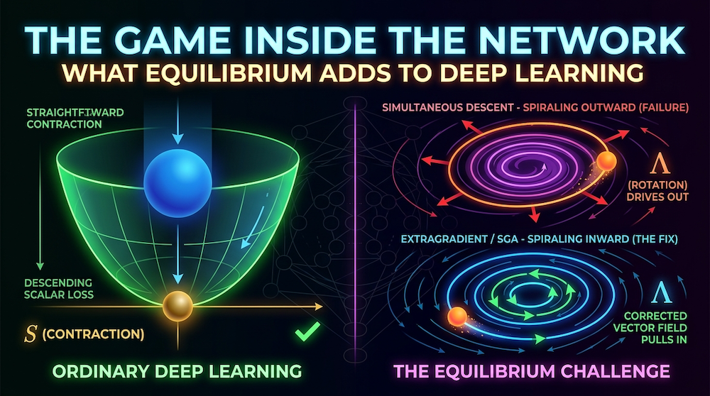
W35 Trend Tutorial | Difficulty: Advanced | Research area: Neural games and multi-agent learning
Modern AI systems increasingly learn from opponents: a generator faces a discriminator, a policy faces earlier versions of itself, and a language model proposes answers that another model scores. It is tempting to call every such loop "self-play." Game theory gives us a sharper question: what game is being played, and what would it mean for learning to settle?
That distinction matters because optimization and equilibrium are not the same thing. In ordinary supervised learning, we minimize one loss against a fixed dataset. In a game, each learner changes the objective seen by the others. The loss surface moves while we optimize it.
This piece is longer than our usual. The material is genuinely new to most practitioners, and the interesting questions — can a neural network's own layers be players? can we co-train a world model's components as a game instead of freezing them one at a time? — only become answerable after the groundwork is laid. We build it in order: equilibrium, the settings beyond zero-sum, the geometry, then the systems.
From one optimum to several best responses
A finite two-player game can be written with payoff matrices and . If the row player uses mixed strategy and the column player uses , their expected payoffs are
A Nash equilibrium is a pair of mutual best responses. Holding fixed, player one cannot improve by changing alone; holding fixed, player two cannot improve by changing alone. This is a stability condition, not a claim that the outcome is fair, globally optimal, or unique.
That last sentence is the first practical lesson. If two neural policies stop changing, we have not proved that they reached equilibrium. They may have collapsed, cycled slowly, or become stuck because gradients vanished. Practitioners therefore measure exploitability or regret: how much could a player gain by switching to a best response?
For player one, one useful diagnostic is
Zero exploitability for every player is the equilibrium condition. A flat training curve is not.
Zero-sum is one setting among several
Zero-sum is where most of us first meet Nash equilibrium, and it is unusually well-behaved: , one player's gain is exactly the other's loss, and von Neumann's minimax theorem guarantees that a value exists and that equals over mixed strategies. Almost every clean convergence guarantee in this literature lives in that world.
It is not the only setting, and for deep learning it is often the wrong one. The taxonomy worth carrying:
General-sum. is unrelated to . Both players can gain, both can lose, and the minimax theorem no longer applies. Equilibria still exist in mixed strategies (Nash's theorem), but the value is not unique, and the comfortable "one number summarizes the game" intuition is gone. Most multi-network training is general-sum, which is precisely why importing zero-sum intuitions is risky.
Common-payoff (fully cooperative). : all players share one objective. This is the degenerate corner where the game collapses back into ordinary optimization — and, as we will see, it is the reason a standard neural network trained on a single loss does not feel like a game.
Potential games. A middle ground: there exists a single scalar function such that every player's unilateral payoff change is mirrored by the same change in ,
Players have different objectives, yet the whole system is secretly descending one function. Potential games converge under simple dynamics. When a multi-network setup is (approximately) potential, ordinary simultaneous gradient descent is fine — and this is a testable property, not a hope.
Stackelberg (bilevel) games. The players are not symmetric: a leader commits first and the follower best-responds. The leader optimizes subject to . This is the right frame for most of the "two networks, one is trained more" setups we actually build — including, as we will argue below, both GANs-in-practice and actor–critic. Fiez, Chasnov and Ratliff (arXiv:1906.01217) give the convergence analysis for the learning dynamics.
Mean-field games. When the player count is large, we stop tracking individuals and track the distribution of players. Each agent best-responds to the population density rather than to named opponents. This is what makes "many players" tractable at all.
The practical upshot: before importing any result, name the setting. A guarantee proved for two-player zero-sum is not evidence about a six-component general-sum training system, and policy gradient has been shown to have no convergence guarantee even in linear-quadratic games (arXiv:1907.03712) — a setting far simpler than any neural one.
Equilibrium is a resting point; co-evolution is a trajectory
Here is a place where the textbook picture and practice genuinely diverge, and the practitioner's instinct is the correct one.
The equilibrium story says: two competitors contest a limited resource, and there is a point at which neither can profitably deviate — both "settle," and the balance holds. That is a statement about a fixed point. What we actually observe when two networks train against each other is usually a trajectory: each keeps finding new weaknesses in the other, each patches them, and the pair ratchets upward in capability without ever coming to rest. Biologists call this Red Queen dynamics — running to stay in place. In our world it is co-evolution, and it is the normal case, not the pathology.
Three corrections follow, and they matter for how we read a training run:
Cycling is not automatically failure. In a zero-sum game the time average of the iterates can converge to equilibrium while the last iterate orbits forever. If we are harvesting a data stream — as in self-play — the orbit is doing useful work: it keeps sweeping the strategy space and generating opponents the learner has not beaten yet. The failure is not motion; the failure is motion that revisits the same states without capability gain.
"Both are happy" is not the same as "both are good." An equilibrium can be reached at a low skill level. Two weak policies that have each stopped finding profitable deviations against each other are at a Nash equilibrium of the game they are playing, and may be trivially beaten by any third policy. This is the single most common way a self-play run lies to us.
Capability and stability are separate axes. A pair can co-evolve to high skill while remaining maximally unstable, or converge beautifully to mutual mediocrity. Any dashboard reporting one number cannot distinguish these.
The engineering response is to stop treating the opponent as a single moving point and start treating it as a population. Policy-Space Response Oracles (arXiv:1711.00832) formalizes this: maintain a pool of policies, compute a meta-distribution over the pool, and train a best response to that mixture rather than to the latest checkpoint. The pool is what converts an aimless cycle into a ratchet, because a new policy must beat the history, not merely today's opponent.
The object we optimize is a vector field
That distinction becomes operational once the players are neural networks. Let and be their parameters and let and be their losses. Single-objective training follows one gradient. Game training follows the joint operator
This is the central conceptual move of the whole field, and it is worth stating plainly: in single-objective learning we descend a scalar function; in a game we follow a vector field that is generally not the gradient of anything. Every intuition we have about loss landscapes — basins, saddles, "the loss went down so we made progress" — is borrowed from a scalar world and does not transfer for free.
The Jacobian exposes why. Decompose it into symmetric and antisymmetric parts:
governs contraction or expansion — the part that behaves like ordinary optimization. produces rotation, and it has no analogue in single-objective training. Balduzzi et al., The Mechanics of n-Player Differentiable Games (arXiv:1802.05642) show this decomposition splits any differentiable game into a potential component (which reduces to gradient descent on an implicit function) and a Hamiltonian component (which obeys a conservation law and circles a fixed point perpetually, exactly like a frictionless pendulum). A game that is purely potential is safe for ordinary gradient descent. A game with a large Hamiltonian component cannot be fixed by tuning a scalar optimizer, because the thing making it fail is not a step-size problem — it is a conservation law.
Reading and without the vocabulary
That decomposition is the diagnostic the rest of this piece leans on, so it is worth making concrete before we use it. Read as the answer to a single question: if we nudge the joint parameter vector, which way does the field push back? The two parts answer two different halves of it.
is the inward/outward part. It behaves like curvature in ordinary training. Positive definite means the field pulls the players back toward the fixed point — a ball in a bowl. This is the part our existing optimizer intuition is actually valid for.
is the sideways part. It pushes perpendicular to any direction that would reduce anything. Nothing in single-loss training produces it. The picture is a marble circling the rim of a frictionless bowl: no energy leaves the system, so it never settles, and no amount of patience makes it settle.
There is also a reading in terms of the players, which is the one worth carrying. The symmetric part is where the two players agree about the cross-effect — the influence of my move on your loss matches the influence of your move on mine — and agreement of exactly that kind is what allows a single scalar function to exist behind the scenes. That is the potential case from the taxonomy above. The antisymmetric part is where they disagree exactly: my gain is your loss, so the cross-terms cancel instead of accumulating into any scalar. Zero-sum is the extreme, which is why zero-sum games are all rotation and no descent.
"Hamiltonian" is borrowed from mechanics, and it means only that a conserved quantity exists. Here that quantity is the squared norm of the field itself,
This is what makes the diagnostic cheap. is one Jacobian-transpose-vector product — a single backward pass through the gradient, no explicit Jacobian, no matrix. And it satisfies an identity that does the measurement for us:
because the antisymmetric part contributes nothing to a quadratic form (). So a single inner product isolates the symmetric part exactly.
It is worth being careful about which way that implication runs, because the tempting reading is the wrong one. What is guaranteed is the forward direction: forces , and forces it negative. The converse does not hold — is a Rayleigh quotient along a single direction, and an indefinite can produce any sign at all. So read it as a one-sided test: a negative value is a certificate that we are not in an attracting region; a positive value is consistent with attraction but does not establish it. A value near zero alongside a large is the interesting case — it says the field has almost no contraction along its own direction, which is motion that is nearly all rotation. That is what "inspect the joint Jacobian" in the checklist below actually cashes out to in code.
Continuous time and discrete time are not the same story
One distinction is worth drawing sharply, because it is where a lot of misapplied theory enters. In continuous time the game flow is , and in a purely Hamiltonian game that flow conserves : trajectories ride level sets forever, in closed orbits. They are neutrally stable — neither converging nor diverging.
Every algorithm we actually run is a discretization of that flow, and discretization is not neutral. Forward Euler with step — which is exactly simultaneous gradient descent-ascent — commits the field evaluated at the start of the interval to the whole interval, and on a curving trajectory that consistently overshoots to the outside of the curve. The local truncation error is not a symmetric wobble; it has a sign, and it points away from the fixed point. The multiplier we are about to derive is precisely that error, accumulated.
So the honest statement is: a conservation law plus forward Euler at any positive step size yields discrete-time divergence. The qualifier matters — this is a fact about that discretization, not about discretization in general, and it is exactly why a better-chosen update rule can recover what Euler destroys. But the moral is general enough to carry: a convergence result proved for the flow does not transfer to the iterates for free, and this is the single most common way a correct theorem gets quoted in support of a false expectation. Extragradient and SGA are best understood not as optimizer tricks but as discretizations chosen so that the leading error term points inward instead.
Their Symplectic Gradient Adjustment (SGA) is the corresponding fix: add a correction term derived from that converts rotation into convergence, with last-iterate guarantees in both the potential and Hamiltonian cases. Crucially, this construction is stated for players from the start, which is what makes it the right tool when we move past two networks.
The bilinear case, worked
In the zero-sum bilinear game , the operator is . Simultaneous gradient descent-ascent gives
Its squared radius evolves as
The matrix has eigenvalues , each with modulus . Therefore, for every nonzero step size, the iterates both rotate and expand: they spiral away from the equilibrium . This conclusion follows from the eigenvalues and the exact radius recurrence, not merely from the matrix determinant. To be precise about the scope of the claim: it is a statement about the iterates produced by this update rule, not about the game being ill-posed. The game itself is perfectly well behaved — the value is and is the unique equilibrium. And note that here even the time average does not rescue us: because the radius grows geometrically, the running mean is dominated by its most recent terms and diverges along with them. This is worth stating because "the time average converges" is a real theorem in this area, but it belongs to no-regret dynamics and to the continuous-time flow , whose orbits are closed circles. Discrete simultaneous steps with are the case that expands. So neither a longer run nor a prettier loss curve fixes the geometry; only changing the update rule does, which is the point of the next section. Note that this game is purely Hamiltonian — , is everything — which is why it is the standard counterexample.
An extragradient step evaluates the field at a look-ahead point before committing the update:
For the bilinear example, the update matrix becomes
whose squared-radius multiplier is when . The look-ahead converts an expanding orbit into a contracting one in this local model. This does not prove convergence for an arbitrary non-convex neural game, but it explains why extragradient and optimistic methods are principled interventions rather than optimizer folklore. Gidel et al. (arXiv:1802.10551) develop the variational-inequality framing that makes this a general recipe rather than a trick for one toy problem.
What this looks like in code
Both interventions are short, and the gap between the equations above and a training loop is smaller than it looks. The one genuinely non-obvious part is getting without ever materializing the Jacobian — so that is the part worth spelling out.
Two helpers are assumed throughout, both mechanical: game_gradient (defined in the second block below) returns the joint field as one flat concatenated vector, and unflatten is its inverse, splitting that vector back into per-parameter shapes. Neither is shown in full, and nothing conceptual hides in them.
Extragradient needs no second-order information at all. It is the same step twice, with the second one evaluated at the look-ahead point:
def extragradient_step(compute_losses, params, eta):
    """One extragradient step. Costs two field evaluations, no curvature."""
    xi = game_gradient(compute_losses(), params)          # F(z_t)
    backup = [p.detach().clone() for p in params]

    with torch.no_grad():                                  # z_{t+1/2} = z_t - eta*F(z_t)
        for p, g in zip(params, unflatten(xi, params)):
            p -= eta * g

    xi_half = game_gradient(compute_losses(), params)      # F(z_{t+1/2})

    with torch.no_grad():                                  # z_{t+1} = z_t - eta*F(z_{t+1/2})
        for p, b, g in zip(params, backup, unflatten(xi_half, params)):
            p.copy_(b - eta * g)
SGA needs , and the trick is that implies
so two Jacobian-vector products suffice. is one ordinary backward pass through the gradient. is the forward-mode product, which reverse-mode autodiff can emulate with the standard double-backward through a dummy variable:
def game_gradient(losses, params):
    """F: each player's gradient w.r.t. its OWN parameters, flattened and concatenated.
    create_graph=True keeps F differentiable so we can take Jacobian-vector products."""
    return torch.cat([
        torch.autograd.grad(L, p, create_graph=True)[0].reshape(-1)
        for L, p in zip(losses, params)
    ])

def sga_direction(losses, params, align=True, eps=0.1):
    """Balduzzi et al. (2018), Algorithm 1. Returns a direction for any optimizer."""
    flat = lambda gs: torch.cat([g.reshape(-1) for g in gs])
    xi   = game_gradient(losses, params)
    v    = xi.detach()

    Jt_xi = flat(torch.autograd.grad(xi, params, grad_outputs=v, retain_graph=True))

    u     = torch.zeros_like(xi, requires_grad=True)       # double-backward gives J @ v
    Jt_u  = flat(torch.autograd.grad(xi, params, grad_outputs=u, create_graph=True))
    J_xi  = flat(torch.autograd.grad(Jt_u, u, grad_outputs=v, retain_graph=True))

    antisym_xi = 0.5 * (Jt_xi - J_xi)                      # Lambda^T F

    if align:
        grad_H = Jt_xi                                     # H = 0.5*||F||^2  =>  grad H = J^T F
        lam = torch.sign(
            (v @ grad_H) * (antisym_xi @ grad_H) / v.numel() + eps
        )
    else:
        lam = 1.0

    return xi + lam * antisym_xi                           # plug into any optimizer
The u line is the one that reliably looks like a bug, so it is worth pausing on. u is initialized to zeros, so Jt_u — the value — really is the zero tensor. That does not matter, because we never use its value. We differentiate it with respect to u, and is linear, so its derivative is the same map at every point, zero included: . The zeros are just a cheap place to evaluate a derivative that does not depend on where it is evaluated. If you would rather not rely on the trick, torch.autograd.functional.jvp computes the same product directly and agrees with these three lines to machine precision; the double-backward is written out here because it composes with an existing graph instead of rebuilding one.
Three details carry most of the practical weight.
The sign of is not cosmetic. The align branch is Balduzzi et al.'s alignment rule, and it exists because a positive speeds convergence toward stable fixed points but can also drive the iterates toward unstable ones. The two inner products are the two checks: probes whether the nearby fixed point is attracting or repelling, and probes whether the adjustment points toward it or away. The is a deliberate weak bias toward stable fixed points when the product is near zero. Setting align=False gives , which is fine on a game already known to be well behaved and wrong in general.
The cost is real but bounded. Extragradient is two field evaluations per step. SGA is one field evaluation plus two Jacobian-vector products — three backward passes per step against a plain step's one, so roughly two to three times the cost in practice, with no storage anywhere. Neither scales with the number of players in any special way: game_gradient already loops over of them, and the decomposition is indifferent to .
Sanity numbers. On these are exactly checkable, and computing them in exact rational arithmetic (rather than floating point) makes the geometry unambiguous. Writing , one step multiplies by:
| Update rule | Multiplier on | At | after 2000 steps, from |
|---|---|---|---|
| Simultaneous GDA | |||
| Extragradient | |||
| SGA, |
Both fixes turn the spiral inward, and on this game SGA turns it inward considerably harder. Here SGA contracts whenever , which at is simply — a comfortably wide range. That bound is a property of this game, though, not a general licence, and the next paragraph is the reason the distinction matters.
One warning the toy example hides. The adjustment is not step-size-neutral: its magnitude scales with , so a strongly rotational game shrinks the usable learning rate. Take Balduzzi et al.'s own weak-attractor example, and . There the field is linear, , with
a weak attractor coupled to a strong rotation. The adjusted field then collapses to something startlingly simple:
The rotation is removed completely — but the effective gain is now , so the update contracts only for . At this is spectacular (the iterates shrink by per step); at it diverges. Re-tune the learning rate after switching on SGA — an unchanged that was stable under plain descent can be unstable under the adjustment, and the failure looks like a bug rather than a step-size problem.
Beyond two: what changes with players
Nothing in the vector-field formulation is specific to two players. For players with parameters and losses , the operator is simply
and the symmetric/antisymmetric decomposition goes through unchanged. This is the sense in which "extend the game to many players" is not merely possible but is the natural generality — the two-player case is the special one, kept for pedagogy.
What genuinely changes at scale is three things. First, equilibria proliferate; selecting among them becomes a design decision rather than a solve. Second, exact equilibrium computation becomes intractable, so we approximate — DNQ (arXiv:2606.06480), which we discuss below, is explicit that its exact -player variant "becomes computationally impractical" while a pairwise decomposition scales. Third, the rotational structure gets richer: with players, can encode cyclic dominance patterns (A beats B beats C beats A) that have no two-player analogue and that no scalar metric will reveal.
For very large , mean-field methods (arXiv:1802.05438) replace named opponents with a population distribution, and the problem becomes tractable again — at the cost of assuming players are interchangeable.
The GAN: two players, opposed objectives, one system that improves
A GAN makes all of this concrete, and it is the cleanest case of "two networks with different objectives that improve because of each other." The original formulation of Goodfellow et al. (arXiv:1406.2661) is a minimax game on a single value function:
For a fixed , the optimal discriminator has a closed form,
and substituting it back reduces the generator's problem to minimizing . The adversary is, in effect, computing a divergence that we do not know how to write down. That is the deep reason the arrangement works: is not helping out of cooperation, it is supplying a learned, adaptive loss function for — one that stays informative as gets better, which a fixed loss cannot do.
Two refinements are worth stating precisely, because both are commonly garbled:
The practical GAN is not zero-sum. Written as above it is. But the saturating generator loss tends to have vanishing gradient when is bad and correctly rejects its samples — precisely when a strong training signal is most needed — so in practice everyone uses the non-saturating variant, maximizing instead. The two players now optimize objectives that are not negatives of each other. The GAN we actually train is a general-sum game, and the zero-sum theory we quote about it is, strictly, about a model we do not run. That does not make the zero-sum formulation useless — it remains the reference object that tells us what the non-saturating variant is an approximation to, and the /JSD derivation above is what explains why the arrangement works at all. The error is not using it; the error is quoting its convergence guarantees as though they applied to the objective we actually optimize.
The discriminator really is the easier problem, and there is a reason. Given , the discriminator faces an ordinary supervised binary classification task against a (momentarily) fixed data distribution — a well-conditioned scalar objective. The generator faces a target that is defined by the other network and moves every time updates. The asymmetry is structural, not an artifact of architecture choice, and it is why the standard practice is discriminator steps per generator step: we are approximating the inner solve of a Stackelberg problem, , in which leads and best-responds.
Mode collapse is the swap of for . The usual gloss — "stuck in a local minimum, producing one mode" — points at the right symptom but the wrong mechanism. If the generator gets to move second against the current discriminator rather than against the best one, its optimal play is to dump all its mass on the single point that today's scores highest. That is a rational best response, not an optimization failure; the run has silently solved instead of , and those differ in a general-sum game. Unrolled GANs (arXiv:1611.02163) attack it directly by differentiating through steps of the discriminator's update, so the generator optimizes against where is going rather than where it is. WGAN (arXiv:1701.07875) attacks it from the other side, replacing JS with a Wasserstein critic that keeps supplying gradient where JS has saturated.
The rest of the game-aware toolkit follows the same logic: alternating updates, regularization, opponent pools, extragradient methods, regret minimization, and explicit exploitability tests. Optimistic Mirror Descent (arXiv:1711.00141), for example, has a last-iterate convergence result for bilinear zero-sum games where ordinary gradient dynamics cycle. The guarantee belongs to that setting, not to every GAN; the transferable lesson is to diagnose the rotational component before tuning a scalar optimizer.
Actor–critic is the same shape with the sign flipped
The resemblance between (generator, discriminator) and (actor, critic) is real, and it has been made formal: Pfau and Vinyals (arXiv:1610.01945) show that GANs can be viewed as actor–critic methods in an environment where the actor cannot affect the reward. Both are bilevel problems in which one network's objective is defined by the other's current output; both are notoriously unstable; and the stabilization tricks — target networks, replay buffers, two-timescale step sizes, gradient penalties — cross over between the two literatures because they are addressing the same structural problem.
But the analogy has a sign error in it that is worth catching, because it changes what we should expect:
- In a GAN, 's objective is opposed to 's. succeeding means scoring worse. The coupling is adversarial.
- In actor–critic, the critic is not an adversary. Its job is to estimate the actor's own value function accurately; a better critic makes the actor better. This is a common-payoff or Stackelberg relationship, not a competitive one — the critic is a learned, self-consistent measurement instrument, not an opponent.
So the correct statement is: GAN and actor–critic share a bilevel structure and an asymmetry in difficulty (in both cases the second player solves a comparatively well-posed regression/classification problem against a target the first player cannot influence), but they differ in the sign of the coupling. "Comparatively well-posed" is a statement about the structure of the second player's problem, not a promise that it is stable in practice: a critic bootstrapping off its own estimates under function approximation and an off-policy distribution can diverge on its own, which is why target networks, regularization, and a slower actor timescale are standard rather than optional. The claim is that the follower's problem is better conditioned given the leader, not that it is unconditionally safe. That difference in sign is why actor–critic's failure modes are estimation failures — value overestimation, the deadly triad, divergence under bootstrapping — while the GAN's are equilibrium failures like mode collapse and cycling. Reaching for the wrong literature's fix is a real and common mistake.
Is a neural network itself a game?
This is the most interesting question in the set, and the answer is yes — with a caveat that explains exactly why it feels counter-intuitive.
The intuition against it is sound: in the idealized case, a standard network has one joint loss, and every parameter is updated to reduce that same scalar. All components go "all-in" on one objective. (Modern systems with auxiliary losses, routing losses, or frozen stages break this assumption — a point we return to immediately below.) In the taxonomy above, that is a common-payoff game, the degenerate corner where the game structure carries no information, because when all payoffs coincide the game-theoretic solution and the optimization solution are the same object. The reason a ResNet does not feel like a game is that it is a game nobody is losing.
And yet the reformulation exists and is non-trivial. Schuurmans and Zinkevich, Deep Learning Games (NeurIPS 2016) construct a reduction of supervised learning to game playing. For convex one-layer problems they establish an equivalence between global minimizers of the training problem and Nash equilibria of a simple two-player game (a protagonist choosing the parameter matrix, an antagonist choosing an affine minorant of the per-example loss). They then extend the construction to general acyclic networks with differentiable convex gates and prove a bijection between the Nash equilibria of the game and the critical (KKT) points of the deep learning problem. The payoff is not just conceptual: because the object is now a game, one can train the network with a game-solving algorithm — they use regret matching — instead of gradient descent.
So the honest answer to "has anyone set up the layers as players and let them co-evolve" is: the equivalence is established and rigorous, and it is a genuinely different lens on what backpropagation computes. What it has not done is displace SGD in practice, and we should say so plainly rather than oversell it.
There is also an engineering version of the idea that is much more widely deployed than the theory. Decoupled Neural Interfaces using Synthetic Gradients (arXiv:1608.05343) breaks the network into modules that update without waiting for the true gradient from downstream, each consuming a predicted gradient from a small auxiliary model. The moment updates are decoupled, the modules are no longer solving one synchronized problem — each is optimizing against a stale or predicted signal from the others, which is precisely a game with imperfect information. The instability that shows up when synthetic gradients are pushed hard is game instability, not optimization noise.
The general principle worth taking away: a multi-component network is a game whenever its components' effective objectives differ. They differ when there are auxiliary losses with their own weights, when a router optimizes load balance while experts optimize task loss (the standard mixture-of-experts arrangement), when adapters are trained against a frozen backbone, or when updates are decoupled or asynchronous. A single joint loss with synchronous updates is the special case that collapses back to plain optimization. Most large systems we build today are not that special case.
Multiple networks, one encoder: the world-model question
This is where the theory earns its keep, because it names a problem that is currently solved by brute force.
The ambition is clear: a world model that predicts video, generates text, and outputs actions, sharing one representation. The standard architectural instinct — one encoder, several task-specific decoders — is right about decoders (different output modalities genuinely need different heads; that part is uncontroversial) and correctly identifies the encoder as the bottleneck. And the reason it is a bottleneck is exactly a game-theoretic one: each decoder's gradient pulls the shared encoder toward a representation that serves its task. Those pulls conflict. The encoder is a shared resource contested by players with different objectives — a general-sum game — which is why the multi-task literature is full of gradient-surgery methods that are, in effect, ad hoc equilibrium selection rules.
Two corrections to the common picture of the current state of the art:
Robot-first pretraining is no longer unavailable, and the public data problem is substantially solved. Open X-Embodiment (arXiv:2310.08864) pools data from 22 distinct robot embodiments, contributed by 21 institutions, covering 527 skills across 160,266 tasks, released publicly in a standardized format. On top of it, Octo (arXiv:2405.12213) and OpenVLA (arXiv:2406.09246) are open generalist policies trained on 800k trajectories and 970k real-world robot demonstrations respectively, and (arXiv:2410.24164) trains a flow-matching policy on a large, diverse corpus spanning single-arm, dual-arm, and mobile-manipulator platforms. Octo in particular is built for exactly the shape under discussion: new sensors, tasks, or robot morphologies are integrated by attaching lightweight encoders and output heads without modifying the pretrained transformer. The "you need to own robots to get robot data" constraint was true not long ago and is now a much weaker limitation than it was.
But the shared-encoder-with-many-heads system is still built by freezing, not by co-training — and that vindicates the underlying worry. V-JEPA 2 (arXiv:2506.09985) is the sharpest illustration. It pretrains a video encoder on over a million hours of internet video, then freezes it and trains a separate action-conditioned predictor (V-JEPA 2-AC) on under 62 hours of unlabeled robot video from the Droid dataset, then deploys it zero-shot for pick-and-place on Franka arms in two labs that contributed no training data — with no task-specific training and no reward. The paper is explicit that separating a frozen encoder from a learned predictor is what modularizes generalization and control. That is precisely the stage-then-freeze pattern: it works, and it is a workaround for the co-training problem, not a solution to it. The same staging appears in DreamerV3 (arXiv:2301.04104), where world model and policy are trained in interleaved phases rather than as one joint objective.
So the picture is: the data barrier has fallen, the frozen-encoder architecture is real and shipping, and genuinely joint end-to-end co-training of a shared encoder against several heterogeneous decoders remains rare. The reason is not compute, it is that the joint object is a general-sum game with a strong rotational component and no reason to converge.
Would game-theoretic co-training actually pay off?
The economic case is straightforward and, we think, correct as stated: staged training means sequential passes over a large corpus, with each frozen stage locking in a representation chosen without knowledge of the tasks that come later. Co-training would mean one pass, a representation shaped by all downstream demands simultaneously, and a much shorter iteration loop. Faster turnaround is a compounding advantage, not merely a cost saving.
We should be careful about how much of that is demonstrated versus argued. What is established:
- The decomposition is real and computable. Given a multi-component system, we can estimate the Hamiltonian versus potential components of the game and know in advance whether ordinary joint gradient descent is likely to work. If a system is approximately potential, co-training needs no special machinery — and this is a measurement, not a guess.
- The corrective algorithms exist and are -player from the start: SGA, extragradient, optimistic updates, two-timescale step sizes.
- The diagnostic exists: exploitability, or in the multi-task case, per-head regret against a head trained freely against a frozen encoder.
What is not established is that this beats staged training at frontier scale. We are not aware of a published result showing a large multi-modal world model co-trained end-to-end via explicit game-theoretic machinery and outperforming the staged pipeline. That is a genuine gap, and it is the kind of gap that is interesting precisely because the theory is mature and the engineering is not.
If we were to attempt it, the sequence we would follow:
- Name the game. Write down each component's actual objective, including auxiliary and regularization terms. If they are all identical, stop — it is plain optimization.
- Measure the antisymmetric energy of the joint Jacobian on a small proxy system, using Hessian-vector products rather than materializing . Large relative to predicts that joint descent will rotate.
- Assign roles. If one component's problem is well-posed given the others (the critic, the discriminator, a decoder given a fixed encoder), make it the follower and give it a faster timescale. Two-timescale schemes are the cheapest intervention that addresses the actual structure.
- Apply the correction only if measurement demands it. SGA and extragradient cost extra gradient evaluations; do not pay for them on a potential game.
- Instrument per-player regret, not just joint loss. The joint loss can fall while one head becomes badly served by the shared encoder.
Self-play is a data engine, not a certificate
Self-play supplies a changing opponent distribution. In AlphaZero-style systems (arXiv:1712.01815), game rules provide an unusually strong verifier: wins, losses, and legal moves are externally grounded. In language-model self-play, correctness may be ambiguous, so a model can generate plausible errors and then reward them.
The Generator–Verifier–Updater decomposition makes this failure easy to see:
- The generator proposes games, trajectories, or answers.
- The verifier scores them.
- The updater changes the policy using those scores.
The 2025 paper Self-Improving AI Agents through Self-Play (arXiv:2512.02731) formalizes self-improvement as a GVU operator and proposes a "Variance Inequality" — a spectral condition that is sufficient, under mild regularity, for the stability of self-improvement. The requirement it expresses is that the combined noise of generation and verification must be small relative to curvature and step size. The paper positions STaR (arXiv:2203.14465), SPIN (arXiv:2401.01335), Reflexion, and AlphaZero as instances of the framework.
We should be precise about the status of that result. It is one theoretical proposal — a sufficient condition, not a characterization — and framing existing systems as instances of it is an interpretive claim, not an empirical validation across those systems. Its value for practitioners is as a design checklist:
- Is the verifier more reliable than the behavior it judges? Ten confident votes from copies of one mistaken judge are not ten independent checks.
- Does the update improve a held-out external measure, not merely the internal reward?
- Are we testing against opponents outside the current training pool?
- Does performance persist when the compute budget and random seed change?
The first question is the one that decides whether a loop is self-improvement or self-confirmation. AlphaZero's verifier is the rules of chess. A language model's verifier is frequently another copy of the generator, and correlated error between generator and verifier is exactly the term the Variance Inequality says must stay small.
Neural networks can amortize the search for low-regret candidates
Classical solvers compute an equilibrium for one payoff table. A neural solver can instead learn a mapping from a game description to a candidate strategy. Condorelli and Furlan, in Deep Learning Across Games (arXiv:2409.15197), trained two networks across randomly generated normal-form games, updating each network to reduce regret against the other network's output. Their experiments show near-equilibrium play across heterogeneous games and a tendency toward risk-dominant equilibria in games with multiple solutions; they do not establish exact convergence to Nash equilibrium.
The useful idea is amortization. We spend training compute once so inference can produce a candidate strategy for a new game quickly. But the network's output remains a candidate: we should calculate regret on the actual payoff matrix rather than treating a softmax vector as self-validating.
Equilibrium selection deserves a note of its own here. When a game has several equilibria, which one a learner lands on is determined by initialization, regularization, and the opponent distribution — not by the game. That makes selection an engineering choice we make implicitly and usually without recording it. Deep fictitious play (arXiv:1903.09376) is one explicit selection mechanism: each player best-responds to the empirical average of opponents' historical play rather than to their current strategy, which damps the rotation described earlier by construction.
In larger sequential games, the same pattern appears with more machinery. A critic estimates state-conditioned payoffs, an equilibrium solver produces a strategic target, and policies imitate that target. DNQ: Deep Nash Q-Network (arXiv:2606.06480) uses this solver-in-the-loop shape for partially observable -player bidding, and reports the tradeoff squarely: a pairwise payoff formulation scales to more agents while the exact -player variant becomes computationally impractical. The approximation buys scale, but it also creates a fidelity question: are pairwise payoff estimates preserving the strategic interactions that matter? A three-way interaction that no pair can represent is invisible to the pairwise method by construction.
What a training trace should reveal
The trace should separate three objects that dashboards often collapse:
- Last iterate: the deployable policy at step .
- Time average: , which may converge in games even when the last iterate cycles.
- Population mixture: a distribution over checkpoints or policies, evaluated against responses outside that population.
Reporting only the average can hide an unusable last policy. Reporting only the last policy can miss convergent no-regret behavior. A production system should declare which object it ships.
Regret is only meaningful against a credible response oracle
In a matrix game, a best response is an exact argmax. In a neural game, computing one may itself require training. Suppose we evaluate a candidate joint policy . For player , an approximate exploitability estimate is
where is the strongest response our search procedure found. This is a lower bound on true exploitability: a weak response learner can fail to discover a profitable deviation and make the target look safer than it is.
That asymmetry deserves emphasis, because it inverts the usual reading of a metric. A low exploitability number is the one we cannot trust — it is equally consistent with a genuinely robust policy and with an attacker that did not try hard enough. A high number is trustworthy: a deviation that was actually found actually exists.
A defensible audit therefore trains several fresh response learners with different seeds and budgets, includes simple scripted attacks, and evaluates on held-out environment states. Plot exploitability against response-compute budget. If the estimate keeps rising as the attacker receives more compute, the earlier "equilibrium" claim was an artifact of an underpowered oracle.
For imperfect-information or sequential games, counterfactual regret minimization (Zinkevich et al., NeurIPS 2007) decomposes global regret into local information-set regrets. Predictive Blackwell approachability (arXiv:2007.14358) connects predictive regret matching to optimistic mirror descent and has materially accelerated solving on standard extensive-form benchmarks. The practical point is not that CFR is universal; it is that the evaluation unit must match the game's information structure. A payoff matrix over final checkpoints throws away histories, observations, and hidden information that may determine whether a deviation is available.
A practitioner's equilibrium checklist
Before calling a neural multi-agent system stable, ask eight questions.
If you only have budget for part of this, the order matters. Questions one, two and seven are the triage set — they are cheap, they are answerable on day one from the training script alone, and between them they decide whether any of the rest applies: if the components turn out to share one loss and update synchronously, question seven ends the investigation and none of the machinery in this piece is needed. Questions four and eight are the ones that decide whether a published number means anything, so they become load-bearing the moment a result leaves the team. Three, five and six are the diagnostic depth to reach for once something is actually misbehaving.
First, name the setting. Zero-sum, general-sum, potential, common-payoff, Stackelberg, or mean-field. Guarantees do not transfer across these, and most real systems are general-sum while most quoted theory is zero-sum.
Second, define the players and payoffs. If the verifier's score is a proxy, name the external metric it is supposed to predict.
Third, define unilateral deviation. What action could one player take while the others stay fixed? Without that counterfactual, "Nash" is only decoration.
Fourth, measure regret against fresh best responses. Evaluation restricted to a closed opponent pool can make a brittle policy look stronger than it is outside that pool — and remember that a low estimate is the untrustworthy direction.
Fifth, separate learning progress from strategic stability. A policy can score higher while becoming more exploitable, or become less exploitable without improving the task metric. Ask separately whether the system is co-evolving (capability rising) and whether it is converging (motion decaying). These are independent, and a healthy self-play run often wants the first without the second.
Sixth, inspect the joint Jacobian or a tractable local approximation via Hessian-vector products. Large antisymmetric energy predicts rotational behavior; optimizer tuning alone is unlikely to remove it. This is the measurement that tells us whether to reach for SGA and extragradient or to leave them alone.
Seventh, check whether the components' objectives actually differ. If a multi-network system has one joint loss and synchronous updates, it is a common-payoff game and none of this machinery is needed. If there are auxiliary losses, frozen stages, routers, or asynchronous updates, it is a real game and should be diagnosed as one.
Eighth, disclose the evaluation object and oracle budget: last iterate, time average, or population mixture; exact or approximate best response; number of seeds; environment holdout; and attack compute. Without those fields, "low regret" is not reproducible.
Game theory does not replace deep learning. It tells us what deep learning is optimizing when the target fights back. Once the dataset is another learner, convergence is no longer just a question about gradients. It is a question about incentives, deviations, and whether any player can still profitably change the game.
Sources
Equilibrium, dynamics and game mechanics
- The Mechanics of n-Player Differentiable Games (arXiv:1802.05642) — Hamiltonian/potential decomposition and Symplectic Gradient Adjustment
- A Variational Inequality Perspective on Generative Adversarial Networks (arXiv:1802.10551)
- Training GANs with Optimism (arXiv:1711.00141)
- Convergence of Learning Dynamics in Stackelberg Games (arXiv:1906.01217)
- Policy-Gradient Algorithms Have No Guarantees of Convergence in Linear Quadratic Games (arXiv:1907.03712)
- Deep Fictitious Play for Stochastic Differential Games (arXiv:1903.09376)
- Regret Minimization in Games with Incomplete Information — CFR, Zinkevich et al., NeurIPS 2007
- Faster Game Solving via Predictive Blackwell Approachability (arXiv:2007.14358)
- Mean Field Multi-Agent Reinforcement Learning (arXiv:1802.05438) — large- games via a population distribution
Neural networks as games
- Deep Learning Games — Schuurmans & Zinkevich, NeurIPS 2016 (PDF) — bijection between Nash equilibria and KKT points of the deep learning problem
- Decoupled Neural Interfaces using Synthetic Gradients (arXiv:1608.05343)
- Deep Learning Across Games (arXiv:2409.15197) — Condorelli & Furlan, amortized neural equilibrium solvers
- DNQ: Deep Nash Q-Network for Partially Observable n-Player Games (arXiv:2606.06480)
GANs and actor–critic
- Generative Adversarial Networks (arXiv:1406.2661)
- Connecting Generative Adversarial Networks and Actor-Critic Methods (arXiv:1610.01945)
- Unrolled Generative Adversarial Networks (arXiv:1611.02163) — mode collapse as the min–max/max–min swap
- Wasserstein GAN (arXiv:1701.07875)
Self-play and self-improvement
- Self-Improving AI Agents through Self-Play (arXiv:2512.02731) — GVU operator and the Variance Inequality
- Mastering Chess and Shogi by Self-Play — AlphaZero (arXiv:1712.01815)
- STaR: Bootstrapping Reasoning With Reasoning (arXiv:2203.14465)
- Self-Play Fine-Tuning — SPIN (arXiv:2401.01335)
- A Unified Game-Theoretic Approach to Multiagent RL — PSRO (arXiv:1711.00832)
World models and shared encoders
- V-JEPA 2: Self-Supervised Video Models Enable Understanding, Prediction and Planning (arXiv:2506.09985) — frozen encoder + action-conditioned predictor
- Open X-Embodiment: Robotic Learning Datasets and RT-X Models (arXiv:2310.08864)
- Octo: An Open-Source Generalist Robot Policy (arXiv:2405.12213)
- OpenVLA: An Open-Source Vision-Language-Action Model (arXiv:2406.09246)
- : A Vision-Language-Action Flow Model for General Robot Control (arXiv:2410.24164)
- Mastering Diverse Domains through World Models — DreamerV3 (arXiv:2301.04104)