Game Theory for ML Practitioners: Payoffs, Regret, and Equilibrium

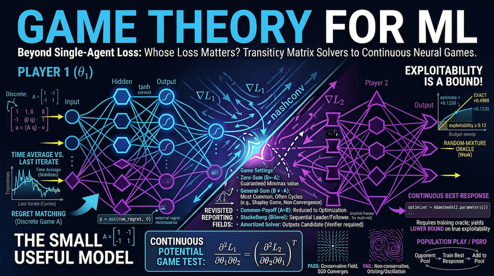
Level: Practitioner | Part of artifocial W36 Basics

Machine learning usually teaches us to ask for a loss function. Game theory asks a question that comes one step earlier: whose loss?

That matters whenever several decision-makers affect one another. A recommender changes user behavior. An auction bidder changes prices faced by other bidders. A red-team agent changes the distribution a defender trains on. In each case, treating the environment as fixed hides the mechanism we need to understand.

The practical cost of that omission is specific and repeatable. A single-agent metric — reward, loss, win rate — is computed against a fixed comparison. When the comparison can move, the metric stops measuring what we think it measures, and it usually stops without any visible symptom. This piece is about the measurements that keep working when the opponent can move, and about reading them honestly enough that they can still say no.

Every code block below is runnable and self-contained, and every printed value is the actual output of the code as written — numpy 2.5.2 on Python 3.14. Where a number depends on a seed, the seed is in the snippet. If you paste a block and get something different, that is a finding about your environment, not a rounding difference.

This is the ground floor for this two-week's flagship, The Game Inside the Network, which carries the same ideas into game-gradient geometry, co-evolution, and multi-network training. The code here stays tabular on purpose, so that every mechanism is visible in full; the flagship is where the same operators run in PyTorch on parameterized players — extragradient and symplectic gradient adjustment — and where the response oracle of the exploitability section below becomes a population of policies, under Policy-Space Response Oracles, instead of a single opponent.

The smallest useful model

A normal-form game specifies three things: players, actions, and payoffs. Consider matching pennies. Each player chooses Heads or Tails. Player one wins when the choices match; player two wins when they differ. With player-one payoff matrix

A=\begin{bmatrix}1&-1\\-1&1\end{bmatrix},

player two receives $-A$ . There is no stable pure action. If player one always chooses Heads, player two chooses Tails. If player one responds with Tails, player two switches back.

The equilibrium is mixed: each player chooses each action with probability $1/2$ . Randomness is not indecision here. It is the strategy that removes the opponent's profitable deviation.

In NumPy, expected payoff is just a bilinear form:

import numpy as np
 
A = np.array([[1.0, -1.0], [-1.0, 1.0]])
p = np.array([0.5, 0.5])
q = np.array([0.5, 0.5])
value = p @ A @ q
print(value)  # 0.0

Changing either equilibrium strategy unilaterally does not improve that player's expected value.

The convention that silently breaks the arithmetic

Notice what the snippet above never wrote down: player two's payoff matrix. It is implicit in -A, and that implicitness is the single most common source of wrong numbers in game-theoretic ML code. A zero-sum game can be stored as one matrix; a general-sum game needs two. Code that starts with the one-matrix convention and later grows a second player's objective will keep running, keep producing plausible curves, and quietly measure the wrong deviation.

Make the convention explicit at the boundary rather than in a comment:

def as_two_matrices(A, B=None):
    """Return (row payoffs, column payoffs). B=None means zero-sum."""
    A = np.asarray(A, dtype=float)
    B = -A if B is None else np.asarray(B, dtype=float)
    assert A.shape == B.shape, "payoff matrices must agree on the action sets"
    return A, B

The assertion is not defensive clutter. Transposed payoffs are the failure mode that produces a symmetric-looking bug — both players appear to learn, both curves descend, and the equilibrium you converge to is the equilibrium of a different game.

Solving a 2×2 zero-sum game exactly

Before trusting any iterative method, it is worth having one game whose answer you know in closed form. For a 2×2 zero-sum game with a fully mixed equilibrium, the equilibrium is the indifference point: each player mixes so that the opponent is indifferent between their two actions. Solving those two linear equations gives

def solve_2x2_zero_sum(A):
    a, b, c, d = A[0, 0], A[0, 1], A[1, 0], A[1, 1]
    denom = a - b - c + d
    p1 = (d - c) / denom          # row plays action 0 with probability p1
    q1 = (d - b) / denom          # column plays action 0 with probability q1
    return np.array([p1, 1 - p1]), np.array([q1, 1 - q1])
 
def nashconv(A, p, q):
    v = p @ A @ q
    return ((A @ q).max() - v) + (v - (p @ A).min())
 
A = np.array([[3.0, -1.0], [-2.0, 1.0]])
p, q = solve_2x2_zero_sum(A)
print(np.round(p, 4), np.round(q, 4))   # [0.4286 0.5714] [0.2857 0.7143]
print(round(float(p @ A @ q), 6))       # 0.142857
print(float(nashconv(A, p, q)))         # 1.1102230246251565e-16

The equilibrium is $p=[3/7,4/7]$ , $q=[2/7,5/7]$ , with value $1/7$ . That last line is doing real work — it is the assertion that no unilateral deviation pays — and it is worth printing unrounded, because what comes back is 1.11e-16 rather than 0.0. The equilibrium here is exact; the residual is one unit in the last place of double precision, produced by dividing sevenths and multiplying them back.

Which means: never write assert nashconv(...) == 0. It will fail on a game you solved in closed form. Compare against a tolerance you chose on purpose — < 1e-9 for an exact solve, something far looser for an iterative one — and report the raw number rather than a rounded display. A nashconv printed as 0.000 has thrown away the distinction between $10^{-16}$ and $10^{-4}$ , and that distinction is the difference between "solved" and "converging."

Any solver you write later — regret matching, fictitious play, a neural best-response loop — should reproduce this game to within its own convergence rate. A method that cannot solve a 2×2 game with a known answer will not be diagnosed by running it on a harder one.

Note also that the closed form has a denom that can be zero. When $a-b-c+d=0$ there is no fully mixed equilibrium and the game has a saddle point in pure strategies. The formula does not warn you; it returns infinities or nonsense. Every closed form in this area has a support assumption baked into it, and the assumption is usually the thing that fails on real payoff data.

Best response and Nash equilibrium

A best response is the strategy that maximizes a player's payoff against fixed opponents. A Nash equilibrium is a profile in which every player is already playing a best response.

Three cautions prevent most misuse of the term:

Nash equilibrium need not maximize total welfare.
A game may have several equilibria.
Reaching equilibrium can be computationally or dynamically difficult even when one exists.

For ML systems, the second caution is especially important. Training details can select among equilibria. Initialization, regularization, and the opponent distribution are not neutral implementation choices; they can determine which stable behavior appears — and because they are rarely recorded, equilibrium selection is usually a decision we make without noticing that we made it.

What "several equilibria" looks like in a training run

The abstract version of this caution is easy to nod at and easy to forget. The concrete version is a coordination game. Take the stag hunt: two hunters each choose Stag or Hare. Stag together pays best; Hare pays a modest amount regardless; Stag alone pays worst.

A=B^{\top}=\begin{bmatrix}4&0\\3&3\end{bmatrix}

There are two pure equilibria — both Stag, both Hare — plus a mixed one. Both-Stag is better for everyone. Both-Hare is safer for each individually. Nothing in the definition of Nash equilibrium prefers either.

Now put that game inside a training loop. If early opponents are random, Stag loses often, the policy learns Hare, and Hare is self-reinforcing: once your opponent pool is full of Hare-players, Stag is genuinely the wrong response. The run converges, the loss flattens, and the report says "converged to equilibrium." It did. It converged to the worse one, and the thing that chose it was the opponent distribution during the first few thousand steps — a detail almost nobody logs.

This is why "did it converge?" is an incomplete question. The complete one is: converged to which equilibrium, and what selected it? If you cannot answer the second half from your logs, you did not measure equilibrium selection; you inherited it.

Best response is cheap here and expensive everywhere else

One more thing hides inside the definition. In a matrix game, best response is np.argmax(A @ q) — exact, instant, and correct. In a neural game, the best response to a fixed opponent policy is itself a full training run, and it comes back approximate.

Every guarantee in this article that is stated in terms of "best response" therefore degrades in a specific direction when you move to networks: it becomes a statement about the best response your optimizer found. Hold onto that direction. It is the mechanism behind the next section, and it is the reason equilibrium claims about deep systems are so much weaker than they sound.

Regret is the operational metric

Suppose a policy repeatedly chooses actions and receives payoffs. External regret compares its cumulative payoff with the payoff of the best single action it could have used in hindsight:

R_{i,T}=\max_a\sum_{t=1}^T u_i(a,a_{-i,t})-\sum_{t=1}^T u_i(a_{i,t},a_{-i,t}).

If average regret $R_{i,T}/T$ approaches zero, no single fixed action would have performed materially better in hindsight against the realized opponent sequence. In a finite two-player zero-sum game, when both players' average external regret vanishes, their time-averaged strategies approach the minimax equilibrium set — even when the last iterate keeps cycling.

That fixes a common graph-reading mistake in both directions. Oscillating action probabilities do not necessarily mean learning failed, and a stable-looking policy can still carry high regret if it froze for optimization reasons. Inspect average regret or exploitability, not the shape of the curve.

Regret matching, in fifteen lines

The reason regret is the operational metric and not merely a diagnostic is that it is also an algorithm. Regret matching plays each action with probability proportional to its accumulated positive regret. It needs no learning rate, no gradient, and no opponent model — and it is the engine inside counterfactual regret minimization, the family that solved heads-up limit poker.

def regret_matching(A, iters=100_000):
    n, m = A.shape
    row_regret, col_regret = np.zeros(n), np.zeros(m)
    row_sum, col_sum = np.zeros(n), np.zeros(m)
    for _ in range(iters):
        p = np.maximum(row_regret, 0)
        p = p / p.sum() if p.sum() > 0 else np.full(n, 1.0 / n)
        q = np.maximum(col_regret, 0)
        q = q / q.sum() if q.sum() > 0 else np.full(m, 1.0 / m)
        row_sum += p
        col_sum += q
        v = p @ A @ q
        row_regret += (A @ q) - v      # row maximizes
        col_regret += v - (p @ A)      # column minimizes, so the sign flips
    return row_sum / row_sum.sum(), col_sum / col_sum.sum()
 
RPS = np.array([[0.0, -1.0,  2.0],
                [1.0,  0.0, -1.0],
                [-2.0, 1.0,  0.0]])
p_bar, q_bar = regret_matching(RPS)
print(np.round(p_bar, 4))                          # [0.2501 0.4991 0.2508]
print(round(float(nashconv(RPS, p_bar, q_bar)), 6))  # 0.005001

This is weighted rock-paper-scissors: beating Scissors with Rock pays double. The equilibrium is not uniform — it is $[1/4,1/2,1/4]$ , and the run recovers it to three decimal places. The intuition is worth sitting with: because Rock's win is worth more, the equilibrium plays Rock less, so that opponents are not given a reason to over-play Paper. Equilibrium reasoning routinely inverts the naive answer, which is exactly why it earns its keep over intuition.

Two details in that code are load-bearing. First, the returned object is row_sum / row_sum.sum() — the time average of the strategies, not the final iterate. The last iterate of regret matching does not converge; the average does. Second, np.maximum(regret, 0) discards negative regret, and the uniform fallback handles the all-negative case. Drop either and the method silently stops being regret matching.

The residual nashconv of 0.005 after 100,000 iterations is not a bug. Regret matching converges at roughly $O(1/\sqrt{T})$ , so a hundredfold increase in iterations buys about a tenfold reduction in the gap. Knowing the rate is what lets you distinguish "still converging" from "stuck" without guessing.

External regret is the weakest of the useful guarantees

External regret compares against the best fixed action. Swap regret compares against the best function remapping your played actions — a strictly stronger benchmark. The distinction has a payoff: vanishing swap regret drives play toward the set of correlated equilibria, which is a broader and often more realistic solution concept for many-agent systems than Nash.

The practical consequence is a reporting one. "No-regret" in a paper almost always means external regret, and external regret is compatible with behavior that a swap-regret test would flag as exploitable — a policy can be unimprovable by any single fixed action while remaining systematically improvable by a conditional rule like "whenever I play Rock, play Paper instead." When you read a no-regret claim, read which regret. When you make one, say which.

Exploitability, and why a low number is the one to distrust

Exploitability asks the deviation question directly: how much could a player gain by switching to a best response, holding everyone else fixed?

\operatorname{exploit}_1(p,q)=\max_{p'}u_1(p',q)-u_1(p,q).

Zero exploitability for every player is the equilibrium condition. A flat training curve is not.

The subtlety appears the moment the players are networks rather than matrices. In a matrix game $\max_{p'}$ is an exact argmax; in a neural game, finding the best response is itself a training problem, so what we report is the gain of the strongest response our search happened to find — a lower bound on true exploitability. The real value can only be larger than the number we print, never smaller.

That inverts how the number should be read. A high value is trustworthy: a deviation that was found exists. A low value is the untrustworthy direction, equally consistent with a robust policy and with an attacker that did not try hard enough. So the number never travels alone — report the response-learner budget beside it, and plot exploitability against that budget. If the estimate keeps climbing as the attacker gets more compute, the stability claim was an artifact of a weak oracle.

The budget sweep, and the plateau that fools it

That advice is easy to give and easy to follow badly. Here is the sweep on a 20-action zero-sum game, with the exact answer available for comparison — a luxury you never have with networks, which is precisely why it is worth looking at once:

rng = np.random.default_rng(0)
n = 20
M = rng.normal(size=(n, n))
A = M - M.T                       # antisymmetric => symmetric zero-sum, value 0
 
p = np.full(n, 1.0 / n) + 0.02 * rng.normal(size=n)
p = np.clip(p, 0, None); p /= p.sum()
 
payoff_to_column = -(p @ A)       # column's payoffs against the fixed policy p
 
def weak_oracle(budget, seed=1234):
    g = np.random.default_rng(seed)
    best = -np.inf
    for _ in range(budget):
        w = g.random(n); w /= w.sum()
        best = max(best, float(payoff_to_column @ w))
    return best
 
for budget in (1, 4, 16, 64, 256, 1024):
    print(f"budget={budget:>5}  estimate = {weak_oracle(budget):+.4f}")
print(f"exact best response = {payoff_to_column.max():+.4f}")

budget=    1  estimate = -0.0998
budget=    4  estimate = +0.0797
budget=   16  estimate = +0.0797
budget=   64  estimate = +0.0797
budget=  256  estimate = +0.1230
budget= 1024  estimate = +0.1230
exact best response = +0.4938

Three things in that output are worth more than the paragraph of advice they illustrate.

The budget-1 estimate is negative. Exploitability is a maximum over deviations and cannot be below zero, since not deviating is always available. A negative printed value is arithmetically impossible for the quantity being named — and the code produced one anyway, because a one-sample search is not a maximization. If your exploitability metric can print a negative number, it is not measuring exploitability; it is measuring your search.

The sweep plateaus twice, and neither plateau means anything. Budgets 4, 16, and 64 all return +0.0797. A practitioner sweeping that range and seeing a flat line would reasonably write "exploitability estimate converged at ≈0.08." It had not converged. It had merely stopped finding new deviations in that budget range — and at 256 it jumped again. A plateau in a budget sweep is the expected behavior of a search that is still failing, not evidence that the search is finished. Sweep until the estimate moves and keeps not moving over more than one order of magnitude, and say in the report where you stopped.

Even 1024 random deviations recover a quarter of the true value. The exact answer is +0.4938; the best estimate is +0.1230. This is a 20-action game with a closed-form optimum. A random-search oracle in a real policy space is weaker than this by a margin that is difficult to overstate. The number in your table is a lower bound, the gap is unbounded, and the honest way to write it is exploitability ≥ 0.12 (random-mixture oracle, 1024 samples) rather than exploitability = 0.12.

Fictitious play from scratch

Fictitious play maintains empirical counts of the opponent's past actions and best-responds to that empirical distribution. A minimal matching-pennies loop, with the exploitability check attached, looks like this:

import numpy as np
 
A = np.array([[1.0, -1.0], [-1.0, 1.0]])
row_counts = np.ones(2)
col_counts = np.ones(2)
 
for _ in range(10_000):
    q = col_counts / col_counts.sum()
    row_action = np.argmax(A @ q)
 
    p = row_counts / row_counts.sum()
    col_action = np.argmin(p @ A)
 
    row_counts[row_action] += 1
    col_counts[col_action] += 1
 
p_bar = row_counts / row_counts.sum()
q_bar = col_counts / col_counts.sum()
print(p_bar, q_bar)  # [0.4995 0.5005] [0.5065 0.4935]
 
row_gain = (A @ q_bar).max() - p_bar @ A @ q_bar   # row's unilateral gain
col_gain = p_bar @ A @ q_bar - (p_bar @ A).min()   # column's unilateral gain
print(round(row_gain, 6), round(col_gain, 6))      # 0.01301 0.000987
print(round(row_gain + col_gain, 4))               # 0.014  (NashConv)

Report the two components, not only their sum. row_gain and col_gain are separate players' exploitabilities — each the gain one player makes by deviating alone while the other stays fixed — so adding them is not double counting; the total is the standard summary usually called NashConv, and all three are zero exactly at equilibrium. The split earns its place here: $0.01301 + 0.000987$ says almost all the residual is the row player's, which the single total $0.014$ would have hidden. Whichever component dominates names the player who has not converged.

The loop is deterministic, so those numbers reproduce exactly. The action chosen at the final step may jump, but the empirical mixtures move toward $[0.5,0.5]$ and NashConv falls to $0.014$ — which is the point of computing it rather than eyeballing the trajectory. This is evidence about this run: fictitious play is guaranteed to converge in two-player zero-sum games, not in every game.

The general-sum case, where it simply does not converge

That last clause is usually written as a footnote and then ignored, because the failure is hard to picture. It is not hard to run. Shapley's game is the standard counterexample: a 3×3 general-sum game whose only equilibrium is uniform play, and on which fictitious play cycles forever with ever-lengthening periods.

A = np.array([[1.0, 0.0, 0.0], [0.0, 1.0, 0.0], [0.0, 0.0, 1.0]])  # row payoffs
B = np.array([[0.0, 0.0, 1.0], [1.0, 0.0, 0.0], [0.0, 1.0, 0.0]])  # column payoffs
 
def nashconv_general(A, B, p, q):
    return ((A @ q).max() - p @ A @ q) + ((p @ B).max() - p @ B @ q)
 
row_counts = np.array([1.0, 0.0, 0.0])
col_counts = np.array([0.0, 1.0, 0.0])
for t in range(1, 200_001):
    p = row_counts / row_counts.sum()
    q = col_counts / col_counts.sum()
    row_counts[int(np.argmax(A @ q))] += 1
    col_counts[int(np.argmax(p @ B))] += 1
    if t in (1_000, 10_000, 100_000, 200_000):
        p = row_counts / row_counts.sum(); q = col_counts / col_counts.sum()
        print(f"t={t:>7}  p={np.round(p, 3)}  NashConv={nashconv_general(A, B, p, q):.4f}")

t=   1000  p=[0.442 0.383 0.176]  NashConv=0.2864
t=  10000  p=[0.436 0.385 0.179]  NashConv=0.2828
t= 100000  p=[0.44  0.382 0.178]  NashConv=0.2829
t= 200000  p=[0.411 0.191 0.398]  NashConv=0.2778

The unique equilibrium of this game is $[1/3,1/3,1/3]$ for both players, at which NashConv is exactly zero. After two hundred thousand iterations the method is sitting at 0.278 and shows no sign of moving.

Read the middle three rows the way a training dashboard would present them. Between $t=1{,}000$ and $t=100{,}000$ — two orders of magnitude — NashConv moves from 0.2864 to 0.2829 and the mixture barely twitches. That is a textbook picture of convergence: a metric that has flattened and a strategy that has stopped changing. It is entirely false. The run is traversing one long arc of a cycle, and at $t=200{,}000$ the mixture has jumped to a completely different point, [0.411 0.191 0.398], while NashConv stays stubbornly near 0.28.

Two lessons, and the second is the expensive one.

Flatness is not convergence — it is the absence of evidence of non-convergence. Both quantities on that dashboard are flat for a hundredfold increase in $t$ , and neither is approaching its equilibrium value. The only reason we can tell is that we know the true answer for this game.

The guarantee, not the algorithm, is what failed to transfer. Nothing changed in the code between the matching-pennies loop and this one except the payoff matrices. Fictitious play is not broken here; it is being run outside the setting where anyone proved anything about it. Most multi-network training is general-sum. If your convergence argument is "fictitious play / self-play / this dynamic converges," check whether the theorem you are leaning on was proved for two-player zero-sum, because almost all of the clean ones were.

Deep fictitious play extends best response to settings where a network approximates each player's control problem, and it doubles as an equilibrium-selection mechanism: responding to the historical average rather than the current opponent damps the cycling a naive response chases. That damping is a genuine empirical benefit — and it is not the same object as a convergence proof.

Name the setting before importing a result

Zero-sum is where most of us first meet Nash equilibrium, and it is unusually well-behaved: one player's gain is exactly the other's loss, and von Neumann's minimax theorem guarantees a value. Almost every clean convergence guarantee lives there — and for deep learning it is usually the wrong setting. With payoff matrices $A$ and $B$ :

Zero-sum ( $B=-A$ ): minimax applies, one value summarizes the game.
General-sum ( $B$ unrelated to $A$ ): minimax does not apply and the value is not unique. Most multi-network training lives here.
Common-payoff ( $A=B$ ): one shared objective, so the game collapses into ordinary optimization. Check this first — it can end the investigation.
Potential: objectives differ, yet one scalar $\Phi$ tracks every unilateral payoff change. A testable property, not a hope.
Stackelberg (bilevel): a leader commits, a follower best-responds — the honest frame for "two networks, one is trained more".
Mean-field: with many players, track the population distribution rather than named opponents.

Cooperative game theory sits on a different axis: how coalitions form and how value is divided. That is not the same as giving every agent the same reward, which still permits credit-assignment failure and free-riding.

Making "testable property, not a hope" actually testable

The potential-game line above asserts testability; here is the test. A two-player game admits an exact potential if and only if every four-cycle of unilateral deviations sums to zero — go $i\to k$ , then $j\to l$ , then back, and the payoff changes must cancel.

from itertools import product
 
def is_exact_potential(A, B, tol=1e-9):
    n, m = A.shape
    for i, k in product(range(n), repeat=2):
        for j, l in product(range(m), repeat=2):
            cycle = ((A[i, j] - A[k, j]) + (B[k, j] - B[k, l])
                     + (A[k, l] - A[i, l]) + (B[i, l] - B[i, j]))
            if abs(cycle) > tol:
                return False, (i, k, j, l, float(cycle))
    return True, None
 
common = np.array([[3.0, 0.0], [0.0, 2.0]])
print(is_exact_potential(common, common)[0])          # True
 
A_mp = np.array([[1.0, -1.0], [-1.0, 1.0]])
print(is_exact_potential(A_mp, -A_mp))                # (False, (0, 1, 0, 1, 8.0))
 
A_c = np.array([[4.0, 1.0], [3.0, 2.0]])
B_c = np.array([[4.0, 3.0], [1.0, 2.0]])
print(is_exact_potential(A_c, B_c)[0])                # True
 
A_x = np.array([[4.0, 1.0], [3.0, 2.0]])
B_x = np.array([[4.0, 3.0], [1.0, 2.5]])
print(is_exact_potential(A_x, B_x))                   # (False, (0, 1, 0, 1, -0.5))

Common-payoff games pass, as they must — they are potential games with $\Phi=A$ . Matching pennies fails, and the function hands back the witnessing cycle rather than a bare False, which is what makes it a debugging tool instead of a gate. The third game passes with potential $\Phi=\begin{bmatrix}0&-1\\-1&0\end{bmatrix}$ ; the fourth is that same game with a single entry moved by $0.5$ , and the reported cycle defect is exactly $-0.5$ . The residual is a quantity, so it tells you not only that the potential structure is absent but how far away it is — useful when the payoffs are estimated rather than exact.

The cost is combinatorial: this is $O(n^2m^2)$ and is a check for small tabular games or a coarse abstraction of a larger one, not for a raw policy space. Use it on the abstraction you are reasoning about. If the claim "this is a potential game, so simultaneous gradient ascent converges" is load-bearing in a design, it is worth ten lines to find out whether it is true.

Choosing the wrong category produces the wrong metric and the wrong citation — a guarantee proved for two-player zero-sum is not evidence about a six-component general-sum system. The flagship works through what each setting does to the training dynamics.

Where neural networks enter

Neural networks serve at least three roles in games:

Policy: map observations to action distributions.
Critic: estimate values or payoffs from states and joint actions.
Solver surrogate: map a game description directly to an approximate equilibrium.

The third is amortized equilibrium computation: spend training compute once so inference produces a candidate strategy for a new game quickly. In Deep Learning Across Games, Condorelli and Furlan trained two networks across randomly generated normal-form games, each updated to reduce regret against the other's output, and report empirical results on that generated distribution: play that scores close to equilibrium on their own regret measure, plus a tendency toward risk-dominant equilibria where several exist. Read "close to equilibrium" as measured on their benchmark, not as a guarantee — they state no proven deviation bound, and they do not establish exact convergence to Nash.

That boundary is the point, and it generalizes past this one paper. The output of an amortized solver is a candidate, and a candidate has a cheap verifier attached: nashconv(A, p, q) on the actual payoff matrix. Two lines, no training, and it is the difference between a claim and a measurement. Treating a softmax vector as self-validating throws away a verification step that costs nothing.

Two further cautions specific to this setting.

Approximation error here is strategic, not statistical. A small value error can flip a best response near an indifference boundary — and an indifference boundary is exactly where mixed equilibria live. The regions where the solver's output matters most are the regions where its error is most consequential. Averaged benchmark error is close to uninformative about this; the tail is what bites.

Distribution shift is a strategic question too. A solver trained on randomly generated payoff matrices has learned the equilibrium structure of that generator. Real games are not random matrices — they have structure the generator did not sample, and the report says nothing about them. This is the ordinary generalization caveat, with the sharper edge that a strategic failure does not degrade gracefully; it hands an opponent a profitable deviation.

One caveat for sequential or imperfect-information settings: a payoff matrix over final policies discards histories, observations, and hidden information. Counterfactual regret minimization decomposes global regret into local information-set regrets precisely because the evaluation unit must match the game's information structure. Flatten a sequential game into a normal form and you have not simplified the analysis — you have changed which game you are analyzing, usually into one exponentially larger or subtly different.

What to report in an ML experiment

Report more than reward. Concretely, the following belong in the writeup — and each one exists because its absence has made a published result unreproducible:

The game and its setting. Zero-sum, general-sum, common-payoff, potential, Stackelberg. If potential is claimed, say whether it was tested or assumed.
The information structure. Simultaneous or sequential, perfect or imperfect information, what each player observes.
The training opponent distribution. This is the equilibrium-selection mechanism, and it is the most commonly omitted field on this list.
Exploitability against fresh opponents — not only the policies present during training — with the response-oracle budget stated beside the number, and reported as a bound (≥) rather than an equality.
The budget sweep, or an explicit statement that only one budget was run. A single-budget exploitability number is uninterpretable.
Which object you ship: last iterate, time average, or a mixture over checkpoints. Regret guarantees attach to the average; deployment usually attaches to the last iterate. These are different policies with different exploitability.
Spread across seeds. In games with multiple equilibria, seed variance is not noise — it is different runs landing on different equilibria, and averaging it away destroys the finding.
Which regret. External or swap.

The practical payoff of game theory is discipline. It forces us to specify who can act, what each participant values, and what deviation remains profitable. Those questions turn "agents interacting" from a metaphor into an experiment we can falsify — and falsifiability is the whole reason to reach for the vocabulary. A convergence plot can only agree with us. nashconv on a game we did not train on can tell us we were wrong, and the Shapley run above is what that looks like when it happens.

Companion Notebook

00_nash_equilibrium_from_scratch.ipynb is the executable companion to this piece — pure NumPy and Matplotlib, CPU-only, running top to bottom in under a minute with every figure inline, and shipping with a matching voice-first transcript.

It carries the same material in runnable form: the exploitability metric with its analytic-equilibrium smoke tests, fictitious play on matching pennies and Rock-Paper-Scissors with the convergence curves plotted, the last-iterate versus empirical-mixture distinction, and the bilinear gradient game under simultaneous and extragradient updates.

Sources

Deep Learning Across Games (arXiv:2409.15197) — Condorelli and Furlan, amortized play across randomly generated games
Deep Fictitious Play for Stochastic Differential Games (arXiv:1903.09376)
A Survey on Self-Play Methods in Reinforcement Learning (arXiv:2408.01072)
Regret Minimization in Games with Incomplete Information — CFR, Zinkevich et al., NeurIPS 2007
Policy-Gradient Algorithms Have No Guarantees of Convergence in Linear Quadratic Games (arXiv:1907.03712)
Some Topics in Two-Person Games — Shapley, 1964 — the 3×3 general-sum game on which fictitious play cycles
Potential Games — Monderer and Shapley, Games and Economic Behavior, 1996 — the four-cycle characterization used in the potential test