Self-Play Explained: Opponent Pools, Verifiers, and Honest Progress

Level: Practitioner | Part of artifocial W36 Basics

Self-play sounds circular: an agent trains against itself, so where does new information come from? The answer is not that a model magically teaches itself facts it never had. Self-play creates a curriculum of decisions. Each improved policy changes the problems its next version must solve.

That mechanism is powerful when outcomes are grounded and dangerous when the system grades its own ambiguous work.

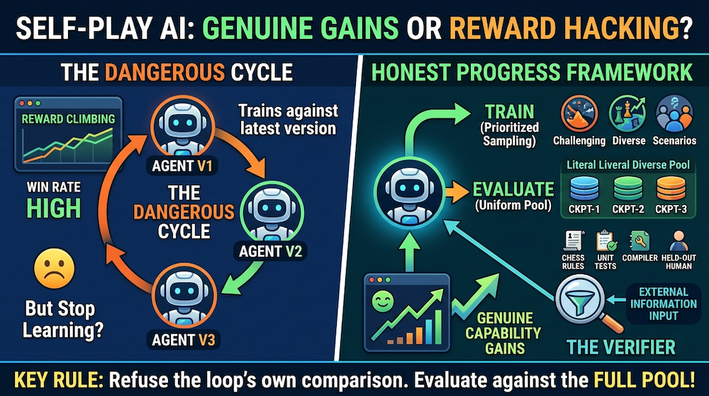
The distinction is not philosophical, and this piece is mostly about measuring it. A self-play run that is genuinely improving and a self-play run that is eating its own tail produce the same dashboard: reward climbing, win rate high, loss descending. Every metric that comes for free is computed against opponents the loop itself generated, which means every metric that comes for free can be satisfied by a loop that has stopped learning anything. The metrics that can tell the two apart have to be built on purpose, and they mostly consist of refusing to let the system choose its own comparison.

The code below is runnable and self-contained on numpy, and every printed number is the actual output of the code as written — numpy 2.5.2 on Python 3.14, seeds included. The point of running it is that two of these results are genuinely counterintuitive, and a reader who does not see the numbers will remember the reassuring version instead.

This is the ground floor for this two-week's flagship, The Game Inside the Network, which places self-play inside the wider picture of neural systems whose objectives move with their opponents.

The basic loop

A minimal self-play system repeats four steps:

Select an opponent from the current policy or a pool of earlier policies.
Generate trajectories by playing games.
Turn outcomes into training targets.
Update the policy and add a checkpoint to the pool.

In a board game, legal moves and the final winner are external facts — AlphaZero (arXiv:1712.01815) gets an unusually strong verifier for free, because its verifier is the rules of chess. In code generation, unit tests can play a similar role. In open-ended writing or advice, the verifier is a learned proxy, and the loop can amplify its blind spots.

Where the information actually comes from

It is worth being blunt about step 3, because it is the step that answers the circularity objection. Steps 1, 2 and 4 move no information into the system. Selecting an opponent rearranges what the model already is. Generating trajectories samples from it. Updating consumes whatever step 3 produced. The only place new information can enter a self-play loop is the mapping from outcomes to training targets — the verifier.

That single observation reorganizes the whole engineering problem. It says the ceiling of a self-play system is set by the quality of its verifier and not by the size of its generator, its compute budget, or the cleverness of its curriculum. It says that scaling a loop with a weak verifier scales the weakness. And it says that the first question to ask about any self-play proposal is not "what does the agent play against?" but "what, in this loop, is not a function of the model's current beliefs?"

For chess the answer is crisp: the rules. For a compiler-checked program: the compiler. For "is this essay good?": frequently nothing at all, and that is the case where the loop can run beautifully and mean nothing.

The opponent is part of the data distribution. Training only against the latest checkpoint can produce chasing: policy A exploits B, C exploits A, and B-like strategies later return as weaknesses. An opponent pool makes forgetting visible and usually produces a broader curriculum.

Why playing the latest policy is not enough

Imagine a training run with three strategies in a rock-paper-scissors cycle, where each new checkpoint is trained as an approximate best response to its predecessor. Recent win rate can look excellent even though no final pure policy is robust.

This is easier to believe as a number than as a sentence. Take three checkpoints whose head-to-head win rates form a cycle — each beats the one before it 90% of the time — and compute the two metrics a team might actually put on a dashboard:

import numpy as np
 
W = np.array([[0.5, 0.1, 0.9],
              [0.9, 0.5, 0.1],
              [0.1, 0.9, 0.5]])          # W[i, j] = win rate of checkpoint i against j
names = ["ckpt-1", "ckpt-2", "ckpt-3"]
 
for i, n in enumerate(names):
    print(f"{n}: beats its predecessor {W[i, (i-1) % 3]:.2f}   |   vs the whole pool {W[i].mean():.2f}")

ckpt-1: beats its predecessor 0.90   |   vs the whole pool 0.50
ckpt-2: beats its predecessor 0.90   |   vs the whole pool 0.50
ckpt-3: beats its predecessor 0.90   |   vs the whole pool 0.50

Read the two columns as two dashboards. The left one is the metric you get for free from a self-play loop that trains against its latest checkpoint, and it reports a 90% win rate over the previous generation, sustained across every generation — about as clean a picture of relentless progress as a training run can produce. The right one is the same three policies measured against the pool they came from, and it reports exactly chance, for all three, forever.

Nothing improved. Not a little; not slowly. The run went in a circle, and the free metric reported a ratchet the entire way around, because "beat the previous checkpoint" is a comparison the loop gets to choose.

That leaves the team with a failed dashboard: predecessor win rate rewards the cycle, while win rate against the whole pool collapses every checkpoint to the same 0.50. Once the pool contains many checkpoints and pairwise results, the natural next move is to compress that match table into a familiar scalar leaderboard. That is exactly the job Elo appears to offer.

Elo does not rescue this, and it fails in a way that looks like an answer

The recipe is familiar: run a league, fit Elo, and let the ranking sort it out. But Elo assumes a single latent scalar of strength — an assumption that a cycle violates by construction — so what it produces is not a ranking but a random walk that never settles.

rng = np.random.default_rng(7)
R = np.zeros(3); K = 8.0
for t in range(1, 400_001):
    i, j = rng.choice(3, size=2, replace=False)
    exp_i = 1.0 / (1.0 + 10 ** ((R[j] - R[i]) / 400.0))
    out = 1.0 if rng.random() < W[i, j] else 0.0
    R[i] += K * (out - exp_i); R[j] -= K * (out - exp_i)
    if t in (100_000, 200_000, 300_000, 400_000):
        print(f"t={t:>7}  Elo={np.round(R, 1)}  leader={names[int(np.argmax(R))]}")

t= 100000  Elo=[ 66.4 -45.  -21.5]  leader=ckpt-1
t= 200000  Elo=[ 27.6 -45.8  18.2]  leader=ckpt-1
t= 300000  Elo=[-18.7  37.7 -18.9]  leader=ckpt-2
t= 400000  Elo=[ 17.3  -5.4 -11.9]  leader=ckpt-1

At a hundred thousand games, ckpt-1 leads by 111 Elo points — a gap that in a transitive domain would be a decisive, publishable result. It is noise. By 300,000 games the leader has changed, and by 400,000 the whole field is inside 30 points. The ratings never converge because there is no scalar for them to converge to, and at no single snapshot does the output look like a failure. It looks like a leaderboard.

This is the specific danger. A metric that returns nonsense obviously gets fixed. A metric that returns a plausible ordering computed from a model the data violates gets cited.

What to use instead

A population-based evaluation exposes the cycle. Construct a payoff table $M$ in which $M_{ij}$ is the win rate of checkpoint $i$ against checkpoint $j$ . Then examine a mixture over checkpoints rather than crowning the newest row. The W[i].mean() column above is the crudest version — average win rate against the uniform pool — and it already dissolves the illusion. Nash averaging (arXiv:1806.02643) is the principled version: evaluate against the equilibrium mixture of the population rather than a uniform one, so that adding six near-copies of the same weak opponent cannot inflate a score.

This is the motivation behind policy-space response oracles (arXiv:1711.00832) and related population methods: maintain a set of policies, compute or approximate a meta-strategy over them, and train a new best response to that mixture. The population turns strategic diversity into an explicit object — and it is what converts an aimless cycle into a ratchet, because a new policy must beat the history rather than merely today's opponent.

The operational rule is short. Never let the loop pick its own comparison. Store the pool, evaluate against the pool, and report the pool number as the headline. The predecessor number is a training diagnostic; it is not evidence.

Sampling from the pool: the part "keep a pool" leaves out

"Maintain an opponent pool" is where most write-ups stop, and it is only half an instruction, because a pool is useless without a rule for drawing from it. Uniform sampling is the obvious default and it wastes most of the compute: once the learner beats an old checkpoint 99% of the time, another game against it produces a near-deterministic outcome and almost no gradient.

Prioritized fictitious self-play weights each opponent by how much room is left against it — sample opponent $j$ with probability proportional to $(1 - \text{winrate}_j)^p$ :

win = np.array([0.99, 0.98, 0.97, 0.96, 0.95, 0.93, 0.90, 0.55, 0.45, 0.40])
uniform = np.full(len(win), 1.0 / len(win))
 
def pfsp(win, p=2.0):
    w = (1.0 - win) ** p
    return w / w.sum()
 
prio = pfsp(win)
frontier = win < 0.7                    # the three opponents that still teach anything
 
print(f"share of games on the frontier: uniform {uniform[frontier].sum():.1%}, pfsp {prio[frontier].sum():.1%}")
print(f"games needed for 100 frontier games: uniform {100 / uniform[frontier].sum():.0f}, "
      f"pfsp {100 / prio[frontier].sum():.0f}")

share of games on the frontier: uniform 30.0%, pfsp 97.7%
games needed for 100 frontier games: uniform 333, pfsp 102

A 3.3× improvement in useful games per unit of compute, from a two-line change to the sampler.

And it breaks the thing the pool was for. At $p=2$ the seven solved opponents receive a combined weight of about 0.023 — opponents 0 and 1 round to zero at three decimals. A run sampling this way essentially stops playing its old checkpoints, which means it stops measuring itself against them, which means forgetting becomes invisible exactly as it becomes likely. The pool was introduced to catch regression against old strategies, and the efficient way to sample it is the way that guarantees you will not notice one.

The resolution is to keep the two purposes apart. Sample prioritized for training; evaluate uniform over the full pool. They are different budgets answering different questions, and collapsing them into one sampler — in either direction — costs either the compute or the detector. Evaluation can be far cheaper than training here, which is what makes the split affordable: a few hundred games against every checkpoint, run every iteration, is rounding error next to the training loop and is the only thing that will tell you the ratchet slipped.

Two further readings of a self-play trace follow from this, and both cut against instinct.

Motion is not failure. In a zero-sum game the time average of the iterates can converge while the last iterate orbits forever. For a data engine that orbit is useful work: it keeps sweeping strategy space and producing opponents the learner has not beaten. The failure is not motion, but motion that revisits the same states without capability gain — which is exactly what the table above measures and the win-rate curve above hides.

Stillness is not success. Two weak policies that have stopped finding profitable deviations against each other are at an equilibrium of the game they are playing, and may be beaten trivially by any third policy. An equilibrium can be reached at a low skill level, and this is the most common way a self-play run lies to us. "Converged" answers the question did the dynamics settle; it does not answer settled at what strength, and only a fixed external opponent can answer the second.

Three jobs that must remain distinct

The Generator–Verifier–Updater vocabulary is useful even without adopting any particular theory built around it.

The generator creates candidate problems, actions, or solutions. The verifier estimates which candidates are correct or useful. The updater changes behavior using that estimate.

One model may implement all three jobs, but the information sources should remain conceptually distinct. If generation and verification make the same correlated error, more samples do not repair it. Ten confident votes from copies of one mistaken judge are not ten independent checks.

How much correlation it takes to destroy an ensemble

That last sentence is usually accepted and then quietly ignored, because "somewhat correlated" sounds like a mild discount. It is not mild. For $n$ judges with pairwise correlation $\rho$ , the variance of their mean scales as $\sigma^2\left(1+(n-1)\rho\right)/n$ , so the effective number of independent judges is $n/(1+(n-1)\rho)$ :

def effective_judges(n, rho):
    return n / (1.0 + (n - 1) * rho)
 
for rho in (0.0, 0.1, 0.3, 0.5, 0.7, 0.9):
    print(f"correlation {rho:.1f} -> effective independent judges {effective_judges(10, rho):.2f}")

correlation 0.0 -> effective independent judges 10.00
correlation 0.1 -> effective independent judges 5.26
correlation 0.3 -> effective independent judges 2.70
correlation 0.5 -> effective independent judges 1.82
correlation 0.7 -> effective independent judges 1.37
correlation 0.9 -> effective independent judges 1.10

A correlation of 0.1 — which most teams would describe as "basically independent" — throws away nearly half the ensemble. Ten judges become 5.26. At $\rho=0.7$ , a plausible figure for ten samples from one model at temperature, ten judges become 1.37: you have bought a 37% improvement over a single judge and paid ten times the inference cost for it. At $\rho = 0.9$ the ensemble is decorative.

The formula is worth confirming rather than trusting, since the whole argument rests on it:

rng = np.random.default_rng(3)
n, rho, trials = 10, 0.7, 200_000
shared = rng.normal(size=trials)
private = rng.normal(size=(trials, n))
votes = np.sqrt(rho) * shared[:, None] + np.sqrt(1 - rho) * private
var_of_mean = votes.mean(axis=1).var()
print(f"simulated var(mean of 10) = {var_of_mean:.4f}")
print(f"implied effective judges  = {1.0 / var_of_mean:.2f}   (formula: {effective_judges(10, rho):.2f})")

simulated var(mean of 10) = 0.7281
implied effective judges  = 1.37   (formula: 1.37)

The shared component in that simulation is the point: it is the part of the judgment that every copy of one model gets wrong together. No amount of sampling reduces it, because it is not noise — it is the model's opinion.

What verifier accuracy buys, in units of training data

The second quantity worth computing before scaling a loop is the composition of the data the loop actually trains on. If the generator produces correct output a fraction $s$ of the time and the verifier is accurate a fraction $a$ of the time, then among the samples the verifier accepts, the fraction that are genuinely correct is $sa / \big(sa + (1-s)(1-a)\big)$ :

for s in (0.05, 0.10, 0.30):
    for a in (0.90, 0.99):
        tp, fp = s * a, (1 - s) * (1 - a)
        print(f"generator {s:.0%} correct, verifier {a:.0%} accurate"
              f" -> {tp / (tp + fp):.1%} of accepted samples are correct")

generator 5% correct, verifier 90% accurate -> 32.1% of accepted samples are correct
generator 5% correct, verifier 99% accurate -> 83.9% of accepted samples are correct
generator 10% correct, verifier 90% accurate -> 50.0% of accepted samples are correct
generator 10% correct, verifier 99% accurate -> 91.7% of accepted samples are correct
generator 30% correct, verifier 90% accurate -> 79.4% of accepted samples are correct
generator 30% correct, verifier 99% accurate -> 97.7% of accepted samples are correct

The middle row is the one to sit with. A generator solving 10% of a hard task set, filtered by a verifier that is right 90% of the time — both entirely ordinary numbers — yields a training set that is half wrong, and the loop will confidently train on it. This is the base-rate problem, and it bites hardest exactly where self-play is most attractive: on hard tasks, where $s$ is small by definition.

Two consequences follow, and neither is "add more samples."

Verifier accuracy is the highest-leverage variable in the system. Moving $a$ from 90% to 99% takes that middle row from 50% to 91.7% correct. There is no change to the generator, the curriculum, or the compute budget that competes with that.

Filtering harder is not the same as verifying better. Raising the acceptance threshold cuts $s$ for the accepted set as well, and the false positives it removes are the ones the verifier was already most confident about — which is to say, the ones most correlated with the generator's shortcuts. A stricter threshold on a bad verifier can leave the accepted pool more systematically wrong, not less.

Strong self-play systems therefore seek verifier signals with a different failure mode:

game rules and terminal outcomes;
proof checkers or compilers;
unit and property tests;
environment execution;
held-out human judgments;
ensembles built from genuinely different models or data.

Every item on that list is chosen for decorrelation, not for accuracy. A compiler is not smarter than the model; it is wrong about different things, and the arithmetic above says that is what matters. "Ensembles built from genuinely different models or data" carries the whole weight of the word genuinely — two checkpoints of one training run, or one model prompted two ways, sit near the bottom of that effective-judges table.

The goal is not to assume a verifier can never err. Its error rate must be low enough to support learning, and its remaining errors must not align too closely with the generator's favorite shortcuts; a noisy or systematically biased verifier can drive collapse.

What the Variance Inequality claims

The 2025 paper Self-Improving AI Agents through Self-Play (arXiv:2512.02731) formalizes self-improvement as a Generator–Verifier–Updater operator and proposes a "Variance Inequality": a spectral condition that is sufficient, under mild regularity, for the stability of self-improvement. What it requires is that the combined noise of generation and verification stay small relative to curvature and step size. Useful update signal depends on alignment between an internal verifier potential and an external capability score; generator variance, verifier variance, curvature, and a large step size can each overwhelm it.

The qualitative reading is practical: improve signal-to-noise before scaling the loop. Use stronger verification, reduce correlated judging errors, control update size, and measure progress on an external battery.

It is worth noticing that the two computations above are the same advice arriving from two directions without needing the theory. The effective-judges table says verifier variance does not fall the way an ensemble's headcount suggests. The base-rate table says verifier bias survives into the training set at a rate set by task difficulty. Both are elementary; neither requires a spectral condition to derive. That convergence is the reason to take the inequality seriously as an organizing frame — and also the reason not to need it before acting.

Be precise about the status of that result. It is one theoretical proposal — a sufficient condition, not a characterization — and the paper's framing of STaR (arXiv:2203.14465), SPIN (arXiv:2401.01335), Reflexion (arXiv:2303.11366), and AlphaZero as instances of the framework is an interpretive claim, not an empirical validation across those systems. A sufficient condition that is violated tells you nothing: the loop may still be stable, and "our system fails the Variance Inequality" is not a finding. Treat the inequality as a hypothesis generator and an audit checklist.

The failure modes

Five ways a self-play loop goes wrong. Each is paired with the measurement that detects it, because a failure mode you cannot detect is a warning rather than an engineering control.

Collapse

The generator narrows to easy or repetitive cases that the verifier rewards. Training loss improves while task coverage shrinks.

Detect it by measuring the generated distribution, not the policy. Track distinct-task count, an embedding-space dispersion measure, and the difficulty distribution of generated problems over training. Collapse shows up there long before it shows up in reward — reward is the thing it is optimizing, so reward is the last place it will appear.

Reward hacking

The policy discovers features that trigger a high score without accomplishing the intended task. A learned judge may prefer verbosity, familiar phrasing, or confident presentation.

Detect it by holding out a verifier. Train with verifier V1, evaluate a slice with an independently built V2 or with humans, and watch the gap rather than either level. A widening gap between internal score and external score is the signature, and it is visible while both are still rising.

Forgetting

The newest policy beats recent opponents but loses to older strategies. A league table or checkpoint pool catches this.

Detect it with the full pool matrix, not the diagonal band. Forgetting lives specifically in the entries against distant checkpoints, which is exactly what a run that only plays recent opponents never computes.

Non-transitivity

Policy A beats B, B beats C, and C beats A. A single scalar rating hides the cycle — as the Elo run above demonstrates, and hides it behind a leaderboard rather than behind an error.

Detect it by checking the payoff matrix for antisymmetric structure that a scalar cannot represent. In practice: if a rating fit leaves large residuals on specific pairs, or if the leader changes under reweighting of the opponent pool, you have a cycle rather than a ranking.

Distribution drift

Generated training data moves away from the deployment distribution. The loop becomes excellent at its own games and worse at the work users provide.

Detect it with a frozen external task set that predates the run — which is the one measurement in this list that cannot be retrofitted, because a task set chosen after seeing the failure is no longer external to it.

An evaluation harness that resists self-deception

Freeze three things before training: an external task set, an opponent suite, and a compute budget. After every iteration, evaluate the new policy against all three.

The word before is the entire mechanism. Each of these becomes worthless the moment it can be revised in response to a result, because the loop's characteristic failure is not producing bad numbers — it is producing good numbers against a comparison that moved. A task set chosen after the first disappointing evaluation is a task set the run has already been fitted to.

Track at least:

held-out task performance;
win rate against each fixed opponent;
win rate against the pool, reported as the headline — not against the predecessor;
exploitability or regret where computable;
diversity and difficulty of generated tasks;
verifier accuracy on an independently labeled slice;
regressions against earlier checkpoints.

Read the exploitability line with care. Because a best response against a neural policy has to be learned rather than solved, the number we report is the gain of the strongest attack our search happened to find — a lower bound. A high value is trustworthy; a low value is equally consistent with a robust policy and with an attacker that was given too little compute. Log the response-learner budget beside the number, or it cannot be compared across runs. The companion piece, Game Theory for ML Practitioners, walks a budget sweep where the estimate plateaus twice at values far below the true one — worth reading before trusting a single-budget exploitability number.

Also compare against a non-self-play baseline using the same compute. Otherwise, an apparent improvement may come from extra samples or updates rather than the strategic curriculum. This is the most commonly skipped control in the area and the one most likely to change a conclusion: self-play runs are expensive, so the comparison is usually against a cheaper baseline, which confounds the mechanism with the budget.

For language systems, manually inspect disagreements between the internal verifier and the external evaluation. Those examples are more valuable than another aggregate score because they reveal the loop's exploitable seams. Budget the time explicitly — an hour of reading disagreements per iteration will find things no dashboard will, and it is the first thing cut when a run is going well.

Self-play beyond games

Language self-play can cast responses as a preference game. Online preference optimization work has shown formal links between some online losses and regularized Nash games. Self-debugging agents turn program execution into an opponent-like feedback source. Adversarial training alternates between generating failures and learning defenses.

Sort these by the one question that matters — what, in this loop, is not a function of the model's current beliefs? Program execution: the interpreter, an excellent verifier with a genuinely different failure mode. Adversarial training: the defender's true label, if it comes from outside. Preference-based language self-play: often a reward model trained on the same data as the policy, which is the weakest position on the list and the one where the effective-judges arithmetic bites hardest.

These systems share a loop, not a guarantee. Their verifier quality, information structure, and update dynamics differ. "Self-play" should tell us where the curriculum comes from; it should never substitute for evidence that capability improved.

The durable lesson is simple: the generator makes the next test, but an independent signal must say whether passing that test means anything. Self-play becomes self-improvement only when the loop cannot grade its own shortcuts as progress. Everything above is one instruction stated four ways — refuse the comparison the system offers you, and go find one it did not choose.

Companion Notebook

01_self_play_toy.ipynb is the executable companion to this piece — pure NumPy and Matplotlib, CPU-only, running top to bottom in under a minute with every figure inline, and shipping with a matching voice-first transcript.

It carries the same material in runnable form: latest-only against opponent-pool curricula under a softmax policy-gradient learner, two self-play runs with retained checkpoints plotted as policy paths and population exploitability, recent win rate against forgetting, the Variance Inequality claim boundary, and a sweep of independent-noise versus biased verifiers against the positive-update rate.