Gaussian Processes Explained: From Kernels to Deep GPs

Level: Intermediate | Part 1 of Artifocial W28 Basics | Research area: Probabilistic machine learning

What Is a Gaussian Process?

Most machine learning models learn a single function from data: they map inputs to outputs via a fixed set of learned parameters. A Gaussian Process (GP) takes a fundamentally different approach. Instead of learning one function, it maintains a probability distribution over an infinite collection of possible functions.

Concretely: a GP is a probability distribution over functions $f : \mathcal{X} \to \mathbb{R}$ such that, for any finite set of inputs $x_1, \ldots, x_n \in \mathcal{X}$ , the joint distribution

$\mathbf{f} = \begin{pmatrix} f(x_1) \\ \vdots \\ f(x_n) \end{pmatrix} \sim \mathcal{N}(\mathbf{m}, \mathbf{K})$

is a multivariate Gaussian. Here $m_i = m(x_i)$ is the mean function evaluated at $x_i$ , and $K_{ij} = k(x_i, x_j)$ is the kernel (covariance) function evaluated at the pair $(x_i, x_j)$ .

We write this compactly as $f \sim \mathcal{GP}(m, k)$ .

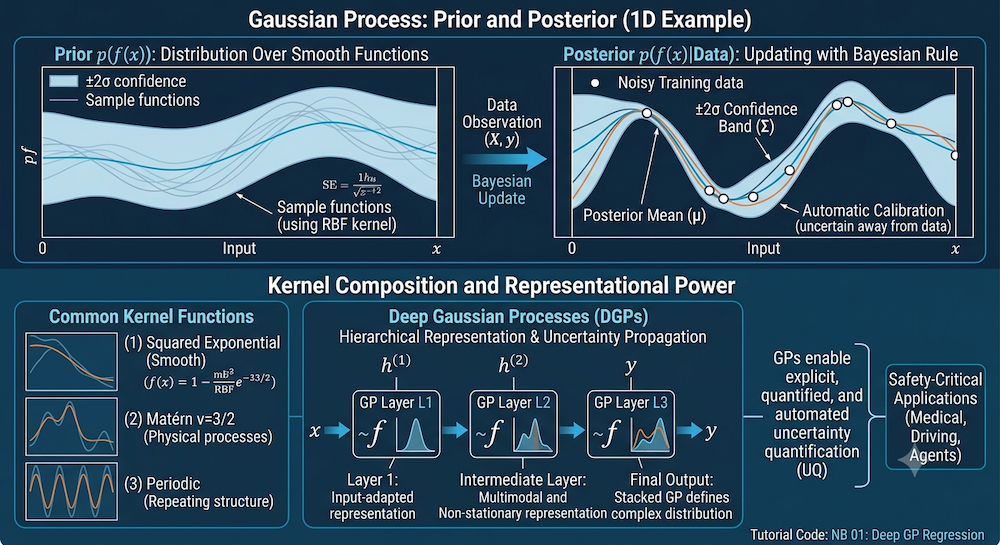
Intuition: before seeing any data, the GP represents our prior beliefs about what $f$ might look like. After seeing observations, we update these beliefs via Bayes' rule to obtain a posterior — a refined distribution over functions consistent with the data.

This is fundamentally different from a neural network, which learns a single function. The GP maintains uncertainty over all plausible functions, giving us not just "what is the prediction" but "how confident should we be in this prediction."

A simple example: suppose we want to model a 1D function from five noisy measurements. Before seeing any data, the GP prior (with an RBF kernel) says "I expect smooth functions." After seeing the data, the GP posterior says "I'm fairly confident the function looks like this in the region where I have data — and uncertain here in the gap between measurements." That uncertainty is explicit, quantified, and automatically calibrated.

Kernel Functions: The Heart of a GP

The kernel function $k(x, x')$ is the central modeling decision in any GP. It encodes our prior beliefs about $f$ : how smooth it is, whether it is periodic, how quickly it varies. Choosing the kernel is choosing the inductive bias.

Why kernels are covariance functions: $k(x, x')$ measures the expected co-variation between $f(x)$ and $f(x')$ . If $k(x, x')$ is large, knowing $f(x)$ tells us a lot about $f(x')$ — the function cannot jump erratically between $x$ and $x'$ . If $k(x, x')$ is small, $f(x)$ and $f(x')$ are nearly independent.

The Squared Exponential (RBF) Kernel

$k_{\text{SE}}(x, x') = \sigma^2 \exp\!\left(-\frac{|x - x'|^2}{2\ell^2}\right)$

$\sigma^2 > 0$ : amplitude — scales the overall magnitude of function values.
$\ell > 0$ : lengthscale — controls how quickly correlations decay with distance.

A small $\ell$ produces rapidly-varying functions; a large $\ell$ produces slowly-varying, smooth functions. The SE kernel produces infinitely differentiable sample paths — very smooth functions. Most introductory GP examples use this kernel.

Matérn Kernels

$k_{\nu}(x, x') = \frac{2^{1-\nu}}{\Gamma(\nu)} \left(\frac{\sqrt{2\nu}|x-x'|}{\ell}\right)^\nu K_\nu\!\left(\frac{\sqrt{2\nu}|x-x'|}{\ell}\right)$

where $K_\nu$ is a modified Bessel function. The parameter $\nu$ controls smoothness:

$\nu = 1/2$ : Ornstein-Uhlenbeck kernel — continuous but nowhere differentiable (Brownian motion-like)
$\nu = 3/2$ : once differentiable
$\nu = 5/2$ : twice differentiable (popular default for physical processes)
$\nu \to \infty$ : recovers the SE kernel

Matérn kernels are widely used for physical and engineering processes that are smoother than Brownian motion but not infinitely smooth.

Periodic Kernel

$k_{\text{per}}(x, x') = \sigma^2 \exp\!\left(-\frac{2\sin^2(\pi|x-x'|/p)}{\ell^2}\right)$

The parameter $p$ is the period. This kernel is useful when the function has repeating structure (seasonal patterns in time series, periodic material properties, etc.).

Kernel Algebra

Kernels can be composed to build richer priors:

Sum: $k_1(x, x') + k_2(x, x')$ — allows functions with multiple types of structure (e.g., a slow trend plus a periodic seasonal component)
Product: $k_1(x, x') \cdot k_2(x, x')$ — models interactions between structures
Composition: $k(h(x), h(x'))$ for a feature map $h$ — allows learned representations (this is exactly what transformer key/query projections do)

The composability of kernels is what makes GPs so expressive as a modeling language. A practiced GP user can often diagnose data structure visually and write down a kernel by inspection.

GP Regression: Prior to Posterior

The setup: we observe noisy data $(X, \mathbf{y})$ where $X = [x_1, \ldots, x_n]^T$ and $y_i = f(x_i) + \epsilon_i$ with $\epsilon_i \sim \mathcal{N}(0, \sigma_n^2)$ . We want to predict $f_*$ at new test points $X_*$ .

Step 1 — Prior: before observing data, our prior is: $f(X) \sim \mathcal{N}(\mathbf{m}_X, K_{XX}), \quad f(X_*) \sim \mathcal{N}(\mathbf{m}_{X_*}, K_{**})$

where $(K_{XX})_{ij} = k(x_i, x_j)$ and $(K_{**})_{ij} = k(x_{*,i}, x_{*,j})$ .

Step 2 — Joint distribution: the joint distribution of noisy training outputs $\mathbf{y}$ and test function values $f_*$ is:

$\begin{pmatrix} \mathbf{y} \\ f_* \end{pmatrix} \sim \mathcal{N}\!\left(\begin{pmatrix}\mathbf{m}_X \\ \mathbf{m}_{X_*}\end{pmatrix}, \begin{pmatrix} K_{XX} + \sigma_n^2 I & K_{X*} \\ K_{*X} & K_{**}\end{pmatrix}\right)$

Step 3 — Posterior: conditioning on the observed data $\mathbf{y}$ using the standard Gaussian conditioning formula yields the posterior:

$p(f_* | X_*, X, \mathbf{y}) = \mathcal{N}(\mu_*, \Sigma_*)$

with closed-form expressions: $\mu_* = \mathbf{m}_{X_*} + K_{*X}(K_{XX} + \sigma_n^2 I)^{-1}(\mathbf{y} - \mathbf{m}_X)$ $\Sigma_* = K_{**} - K_{*X}(K_{XX} + \sigma_n^2 I)^{-1}K_{X*}$

Interpretation:

$\mu_*$ : the posterior mean — our best prediction at test points $X_*$ .
$\Sigma_*$ : the posterior covariance — our uncertainty. The diagonal entries $\Sigma_{*,ii}$ are the marginal variances at each test point.

Key insight: $\Sigma_* \leq K_{**}$ in the positive-semidefinite sense — observing data always reduces uncertainty. Near observed data points, $K_{*X}(K_{XX} + \sigma_n^2 I)^{-1}K_{X*} \approx K_{**}$ , so $\Sigma_* \approx 0$ . Far from data, both terms are small and $\Sigma_* \approx K_{**}$ — we fall back to the prior.

This automatic uncertainty behavior — confident near data, uncertain away from data — is what makes GPs naturally calibrated.

Companion Notebook

NB 01: Deep GP Regression walks through:

Fitting a single GP to a toy 1D dataset with an RBF kernel
Plotting the posterior mean and ±2σ confidence bands
Showing how posterior variance grows away from training data
Fitting a DGP and comparing to the single-layer GP

The Scalability Problem

The central computational challenge of GP regression is the matrix inversion $(K_{XX} + \sigma_n^2 I)^{-1}$ . For $n$ training points, this requires:

Storage: $O(n^2)$ to store the $n \times n$ kernel matrix
Computation: $O(n^3)$ for the Cholesky decomposition used in the solve

For small datasets ( $n \leq 10^4$ ), this is tractable. For large datasets ( $n > 10^5$ ), exact GP inference becomes prohibitive. This scalability barrier kept GPs out of large-scale applications for decades.

Sparse GP approximations address this by introducing $m \ll n$ inducing points $Z = \{z_1, \ldots, z_m\}$ in the input space. The full kernel matrix is approximated via:

$K_{XX} \approx K_{XZ} K_{ZZ}^{-1} K_{ZX}$

This reduces computational complexity to $O(nm^2 + m^3)$ — linear in $n$ for fixed $m$ .

The inducing point locations $Z$ and all kernel hyperparameters ( $\ell$ , $\sigma^2$ , $\sigma_n^2$ ) are learned by maximizing the variational ELBO:

$\mathcal{L} = \mathbb{E}_{q(f)}[\log p(\mathbf{y} | f)] - \text{KL}(q(f) \| p(f))$

GPyTorch (Gardner et al. 2018) implements all of this in PyTorch with GPU acceleration. It uses conjugate gradient (CG) solvers instead of Cholesky decomposition, achieving near-linear scaling in practice and handling millions of data points on modern hardware.

Deep Gaussian Processes

A single GP defines a distribution over functions with a fixed kernel structure. What if the function has hierarchical structure — features at multiple scales, non-stationary behavior, or multimodal uncertainty?

Deep GPs stack $L$ GP layers:

$h^{(1)} = f^{(1)}(x), \quad h^{(\ell)} = f^{(\ell)}\!\left(h^{(\ell-1)}\right), \quad \ldots, \quad y = f^{(L)}\!\left(h^{(L-1)}\right) + \epsilon$

where each $f^{(\ell)} \sim \mathcal{GP}(m^{(\ell)}, k^{(\ell)})$ . The composition of GPs allows the model to represent functions that a single GP with any fixed kernel cannot — for example, functions that are smooth in some regions and rough in others (non-stationarity), or functions with multiple modes of uncertainty.

Why stacking helps:

Layer 1 can learn a low-level, input-adapted representation
Layer 2 composes that representation to capture higher-level structure
Each GP layer provides a principled uncertainty estimate that propagates forward

Training DGPs requires approximation because the intermediate layer outputs are random variables that cannot be marginalized out analytically. The doubly stochastic variational inference (DSVI) approach of Salimbeni & Deisenroth (2017) approximates the ELBO using inducing points at each layer and Monte Carlo estimation of the expectations across layers.

The companion notebook NB 01 builds a 2-layer DGP from scratch in pure NumPy using a custom TwoLayerDeepGP class — no external GP library required. For GPU-accelerated production use, GPyTorch provides DeepGP and DeepGPLayer classes that implement the same architecture with DSVI at scale. Key hyperparameters include the number of inducing points per layer, the dimensionality of intermediate representations, and the kernel at each layer.

A useful intuition: a DGP is to a GP what a deep neural network is to a linear model. Depth adds representational power. But unlike a deep neural network, each layer of a DGP is a full probabilistic model — it outputs a distribution, not a point estimate. Uncertainty propagates through the stack, and the final prediction comes with a calibrated confidence estimate.

Why This Matters for AI

Gaussian Processes are not a historical curiosity from statistics textbooks. They represent a principled approach to uncertainty quantification that modern deep learning has largely bypassed — and is now beginning to rediscover.

The NTK connection (covered in depth in the W28 Trend Tutorial) shows that deep neural networks are implicitly doing something very GP-like. The question is whether we want to make that structure explicit — and pay the computational cost of principled inference — or let it remain implicit and lose calibrated uncertainty.

For safety-critical applications, calibrated uncertainty is not optional:

Medical diagnosis: a model that says "97% confident: benign" on an unusual scan is dangerous if that confidence is miscalibrated.
Autonomous driving: a perception system must distinguish "I'm sure that's a pedestrian" from "I'm not sure what that is."
Agentic AI: an agent taking multi-step actions must know when to act and when to ask for clarification.

This connects directly to the arc ahead: the next entry in this series applies GP-style uncertainty to probabilistic 3D geometry; further entries connect to neuro-symbolic reasoning under uncertainty and close with a probabilistic world model that plans rationally under uncertainty. GPs are the foundation. The arc is about building the full probabilistic stack.