Attention Is All You Need... Is a Kernel

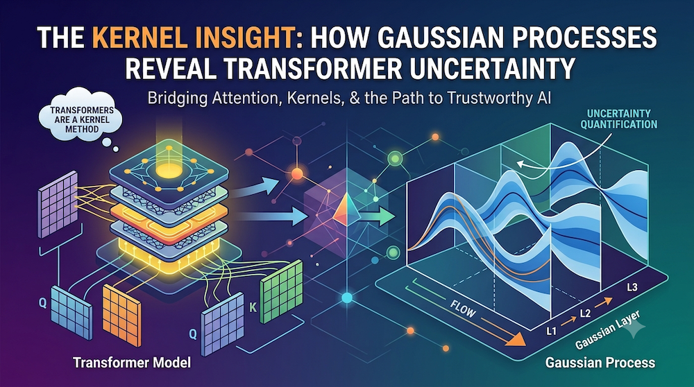
W28 Trend Tutorial | Difficulty: Advanced | Research area: Probabilistic machine learning

The Kernel Insight

In 2017, Attention Is All You Need changed everything. But buried inside the transformer paper — and noticed by almost nobody at the time — is a connection that took the research community years to fully appreciate: if you squint at scaled dot-product attention, it is doing exactly what a Nadaraya–Watson kernel estimator does.

This is not a metaphor. It is a precise mathematical equivalence with profound consequences for how we understand what transformers are, what they are learning, and what they cannot do.

Let us start with the mechanics. Scaled dot-product attention computes, for a query $q_i$ and a set of keys $k_1, \ldots, k_n$ with corresponding values $v_1, \ldots, v_n$ :

$\text{Attn}(q_i, K, V) = \sum_j a_{ij} v_j, \quad \text{where} \quad a_{ij} = \frac{\exp(q_i k_j^T / \sqrt{d})}{\sum_{j'} \exp(q_i k_{j'}^T / \sqrt{d})}$

The weights $a_{ij}$ are softmax-normalized inner products between the query and each key. Now compare this to the Nadaraya–Watson (NW) kernel estimator:

$\hat{f}(x) = \frac{\sum_i K(x, x_i) y_i}{\sum_i K(x, x_i)}$

where $K(x, x_i)$ is a kernel function measuring similarity between $x$ and $x_i$ .

Define $K(q_i, k_j) = \exp(q_i k_j^T / \sqrt{d})$ . Then:

$a_{ij} = \frac{K(q_i, k_j)}{\sum_{j'} K(q_i, k_{j'})}, \quad \text{Attn}(q_i, K, V) = \sum_j a_{ij} v_j$

This is exactly the NW estimator with $x = q_i$ , $x_i = k_j$ , $y_i = v_j$ . Attention is kernel regression. The values are the regression targets. The queries are test points. The keys define how much each training point contributes. The softmax normalizes the kernel.

Tsai et al. (2019) were among the first to make this connection explicit, showing that self-attention can be viewed as a form of kernel method where the kernel is learned rather than fixed. The difference from a classical NW estimator is crucial: the query and key projection matrices $W_Q$ and $W_K$ are trained end-to-end, allowing the model to discover which kernel best captures the task's inductive structure.

This insight immediately raises a question: if transformers are doing kernel regression, what is the underlying probabilistic model? The answer leads us directly to Gaussian Processes.

What Is Kernel Regression? A Quick Primer

Before we reach the GP connection, let us spend a moment on kernel regression — because it is one of those ideas that is simultaneously very old and very deep.

The Nadaraya–Watson estimator was proposed independently by Nadaraya and Watson in 1964. Given training data $\{(x_i, y_i)\}_{i=1}^n$ , the estimator predicts at a new point $x$ as:

$\hat{f}(x) = \frac{\sum_{i=1}^n K(x, x_i) y_i}{\sum_{i=1}^n K(x, x_i)}$

The kernel $K(x, x')$ is a non-negative function that measures similarity. Points close to $x$ contribute more; distant points contribute less. The result is a weighted average of training targets, weighted by proximity.

Common kernel choices:

Radial Basis Function (RBF) / Squared Exponential: $K_{\text{RBF}}(x, x') = \sigma^2 \exp\!\left(-\frac{|x - x'|^2}{2\ell^2}\right)$

The lengthscale $\ell$ controls how quickly weight decays with distance. The amplitude $\sigma^2$ scales the overall magnitude.

Polynomial kernel: $K_{\text{poly}}(x, x') = (x \cdot x' + c)^d$

Linear kernel: $K_{\text{lin}}(x, x') = x \cdot x'$

Notice: attention uses the exponential dot-product kernel $K(q, k) = \exp(q \cdot k / \sqrt{d})$ , not a linear kernel. The exponential is what the softmax applies — it takes inner products and exponentiates before normalizing. The softmax is doing the same job as the NW normalization denominator, but the kernel is $e^{q \cdot k / \sqrt{d}}$ , not $q \cdot k$ itself.

The deeper point is that kernel choice encodes an inductive bias. A short-lengthscale RBF kernel assumes the function varies rapidly; a long-lengthscale RBF assumes slow variation. In transformers, this kernel is parameterized by the projection matrices, allowing the model to learn which inductive bias best suits the data.

This is a key advantage of learned kernels over fixed ones. But it comes at a cost: we lose the principled uncertainty quantification that kernel methods provide when grounded in a probabilistic framework. And that is where Gaussian Processes come in.

From Kernels to Gaussian Processes

A Gaussian Process (GP) is a probability distribution over functions. Formally, a collection of random variables $\{f(x) : x \in \mathcal{X}\}$ is a GP if, for any finite set of inputs $x_1, \ldots, x_n$ , the joint distribution

$\begin{pmatrix} f(x_1) \\ \vdots \\ f(x_n) \end{pmatrix} \sim \mathcal{N}(\mathbf{m}, \mathbf{K})$

is multivariate Gaussian, where $m_i = m(x_i)$ is the mean function and $K_{ij} = k(x_i, x_j)$ is the kernel (covariance) function.

We write $f \sim \mathcal{GP}(m, k)$ .

The kernel function is the heart of the GP: it encodes what functions we a priori believe are plausible. An RBF kernel says "we expect smooth functions." A Matérn-1/2 kernel says "we allow rougher, continuous-but-jagged functions." The kernel is the prior.

The bridge from attention to GPs. If attention is kernel regression, what is the "prior" in the GP sense? This question was crystallized by the Neural Tangent Kernel (NTK) theory of Jacot et al. (2018). The key result: in the limit of infinite width, a neural network initialized with standard random weights behaves as a GP with a specific kernel — the NTK. Training an infinitely-wide network with gradient descent is equivalent to performing GP regression with this kernel.

This is extraordinary. It tells us that the implicit prior of a neural network corresponds to a GP prior with the NTK. For finite-width networks (including all practical transformers), the NTK relationship is only approximate. What we lose at finite width is calibrated uncertainty — we no longer have an explicit posterior variance telling us where the model is uncertain.

The GP posterior. Given noisy observations $y_i = f(x_i) + \epsilon_i$ where $\epsilon_i \sim \mathcal{N}(0, \sigma_n^2)$ , the GP posterior at test points $X_*$ is:

$p(f_* | X_*, X, y) = \mathcal{N}(\mu_*, \Sigma_*)$

with closed-form expressions: $\mu_* = m(X_*) + K_{*X}(K_{XX} + \sigma_n^2 I)^{-1}(y - m(X))$ $\Sigma_* = K_{**} - K_{*X}(K_{XX} + \sigma_n^2 I)^{-1} K_{X*}$

The mean $\mu_*$ is the best prediction. The covariance $\Sigma_*$ tells us how uncertain we are — it is large where data is sparse, small where data is dense. This principled, data-density-aware uncertainty estimate is what attention cannot give us directly.

Deep Gaussian Processes: The Revival

A single GP is powerful but limited. By construction, it is parameterized by a kernel defined on the input space. This means it can only represent functions with the properties encoded by that kernel — smooth functions if we use an RBF, etc.

What if we stacked GPs the way we stack layers in a deep network?

That is the idea behind Deep Gaussian Processes (DGPs), introduced by Damianou and Lawrence (2013). A DGP with $L$ layers defines:

$f = f^{(L)} \circ f^{(L-1)} \circ \ldots \circ f^{(1)}$

where each $f^{(\ell)} \sim \mathcal{GP}(m^{(\ell)}, k^{(\ell)})$ . The output of each layer becomes the input to the next. This composition of GPs allows DGPs to represent non-stationary and multimodal functions that a single-layer GP cannot capture — just as deep neural networks capture hierarchical representations that shallow networks miss.

The catch: DGPs are computationally intractable. Marginalizing out the intermediate layer outputs requires integrating over an exponentially large space. For years, this tractability barrier kept DGPs as a theoretical curiosity.

Two breakthroughs unlocked the revival:

(1) Doubly Stochastic Variational Inference. Salimbeni & Deisenroth (2017) showed that DGPs can be trained via a doubly stochastic variational lower bound. The key idea: introduce inducing points at each layer (a sparse approximation of the GP) and use Monte Carlo samples to estimate the variational ELBO. This makes DGP training scalable to datasets of moderate size.

(2) Scalable GP Libraries. Wilson & Nickisch (2015) introduced KISS-GP (Kernel Interpolation for Scalable Structured Gaussian Processes), which approximates kernel matrices using structured grids and fast matrix-vector multiplication. Later, Gardner et al. (2018) built GPyTorch on PyTorch, leveraging GPU acceleration and conjugate gradient solvers to scale GP inference to millions of data points.

Together, these advances transformed DGPs from theory into practice. We can now train multi-layer GP models that provide:

Hierarchical representations: like deep networks, DGPs learn features at multiple scales
Calibrated uncertainty at every layer: unlike deep networks, each layer propagates uncertainty forward
Principled priors: the GP framework makes our assumptions explicit and modifiable

The parallel with deep transformers is striking: a DGP is to a GP what a transformer is to a single-layer attention mechanism. Both add depth to overcome the representational limits of their shallow counterpart. But where transformers lose principled uncertainty quantification, DGPs preserve it.

Uncertainty Quantification: The Missing Ingredient

Let us be precise about what standard transformers give us and what they do not.

A transformer trained on a classification task outputs logits, passed through softmax to produce a probability distribution over classes. A transformer trained on regression outputs a point estimate. In both cases, the model gives us a prediction — but not a principled measure of how confident it is in that prediction.

This distinction matters enormously in practice. A model might output $p(\text{cat}) = 0.97$ — but if that input is far from anything in the training distribution, that 97% is meaningless. The model has no way to say "I've never seen anything like this; I don't know."

Two types of uncertainty:

Epistemic uncertainty (model uncertainty): arises from limited data. We do not know which function generated the data; the posterior is spread over many plausible functions. This uncertainty can be reduced by collecting more data. In a GP, epistemic uncertainty appears as high posterior variance in regions with few observations.

Aleatoric uncertainty (irreducible noise): the world is inherently noisy. Even with infinite data, some outcomes remain unpredictable. In a GP, aleatoric uncertainty is captured by the noise variance $\sigma_n^2$ .

GPs separate these naturally. The posterior variance $\Sigma_*$ captures epistemic uncertainty; $\sigma_n^2$ captures aleatoric uncertainty. For a standard transformer, neither is directly available.

Expected Calibration Error (ECE) is the standard metric for measuring calibration. If a model says "80% confidence" on 100 examples, a well-calibrated model should be right roughly 80 times. Formally:

$\text{ECE} = \sum_{b=1}^B \frac{|B_b|}{n} \left| \text{acc}(B_b) - \text{conf}(B_b) \right|$

where $B_b$ are confidence bins. Guo et al. (2017) famously showed that modern neural networks are poorly calibrated — their confidence does not match their accuracy, and larger models are often more overconfident.

GPs are naturally well-calibrated under Gaussian noise assumptions. Their uncertainty is directly tied to data density: high where data is sparse, low where data is dense. No post-hoc calibration (e.g., temperature scaling) is required.

The Probabilistic Renaissance: Why Now?

The GP–Transformer duality is not just an academic curiosity. It is a signpost toward what comes next.

For much of the 2020s, the dominant paradigm was scale: more parameters, more data, more compute. Scaling laws suggested bigger models were reliably better. And they were — up to a point.

But several failure modes have accumulated:

Overconfident predictions in out-of-distribution settings (hallucination in LLMs is, in part, a calibration failure)
Inability to reason about uncertainty (a world model that assigns equal confidence to "the obstacle is a pedestrian" and "the obstacle is a shadow" is dangerous)
Brittleness at distribution shift (models trained on clean data fail on corrupted inputs in ways that calibrated uncertainty would flag)

The probabilistic renaissance is a recognition that the statistical machinery abandoned in the race to scale — Gaussian Processes, Bayesian neural networks, variational inference — contains exactly the tools needed to address these failure modes.

The timing is right for several reasons:

Scalable variational inference. The DSVI framework, combined with GPyTorch's GPU-accelerated inference, has made deep probabilistic models practical at the scale of real datasets.

Architectural convergence. The NTK/kernel connection shows that transformers and GPs are not competing paradigms — they are different points in a spectrum. Hybrid architectures are emerging that incorporate GP-style uncertainty heads on top of transformer backbones.

World models demand uncertainty. The push toward autonomous systems — self-driving cars, robotic manipulation, agentic AI — requires models that know what they do not know. This connects to W13's JEPA framework: the Joint Embedding Predictive Architecture learns an implicit energy landscape over world states, and the regions of high energy are exactly where the model is uncertain. JEPA-style models need calibrated uncertainty to be actionable.

Hardware. The same GPU acceleration that made transformers practical now makes variational DGP training practical. The bottleneck was never primarily algorithmic — it was hardware. That bottleneck has lifted.

The arc ahead:

This tutorial establishes the theoretical foundation: attention as kernel regression, GPs as principled probabilistic extensions, DGPs as their deep generalization.

Coming up in this series: probabilistic 3D geometry — moving beyond Gaussian Splatting's point estimates to representations with explicit shape uncertainty.

Further in the series: neuro-symbolic reasoning — how uncertainty quantification enables reliable compositional inference.

Closing the arc: probabilistic world models that plan under uncertainty, using calibrated predictions to distinguish "I know this is safe" from "I don't know enough to act."

The kernel insight is the key that opens all of this. Transformers were probabilistic models all along. We are just now beginning to build them that way on purpose.

Companion Notebooks

Two pure-NumPy notebooks accompany this tutorial:

NB 00: GP Attention from Scratch — proves the NW = attention equivalence numerically (max difference $<10^{-10}$ ), builds the full GP posterior from scratch using Cholesky decomposition, and sharpens the GP-vs-NW distinction as the noise shrinks: the GP mean solves the full kernel system, so as $\sigma_n \to 0$ it interpolates the training data, whereas Nadaraya–Watson — and therefore attention — is a local weighted average whose weights sum to 1 and so never passes through the data (cousins, not twins). It closes on the missing variance column: attention outputs only the mean, the GP gives mean and calibrated uncertainty bands.
NB 01: Deep GP Regression — builds a custom NumPy TwoLayerDeepGP with an input-warping layer, demonstrates shallow GP failure on a non-stationary regression problem (slow sine on the left, fast oscillation on the right), and compares shallow vs deep GP on both MSE and a reliability diagram. (Production-scale equivalent: GPyTorch with DeepGP/DeepGPLayer.)

This tutorial is part of the Artifocial research-multimodal series. Previous: W16 Trend Tutorial — 4D Gaussian Frontier. Next in this series: Probabilistic 3D.